Most “model compression” tutorials stop at a number on a slide — “4× smaller, 1% accuracy drop.” This project is the messier, more honest version: I took a heavyweight ResNet50, taught it two jobs at once (classify a cat’s breed and draw a box around its head), then ran it through the full compression pipeline — fine-tune → prune → quantize — and measured what actually happened at each step.

The headline result: the final model is ~19 MB at ~0.90 breed accuracy — a 5× size cut from the 104 MB baseline. But the interesting part isn’t the headline — it’s the places my intuition was wrong, which is where most of the learning lived. I’ve kept those corrections in the post.

The three axes, and which lever moves which

Compression isn’t one knob. It’s three independent axes — model size (bytes), latency (throughput / FLOPs), and accuracy — and the entire skill is knowing which lever moves which axis, and what it costs. That framing is worth internalizing before any code:

Lever	Size	Latency	Cost
Efficient architecture (MobileNet)	small natively	fast natively	lower capacity ceiling
Unstructured pruning	only via sparse storage / gzip	no win without sparse kernels	best accuracy retention
Structured (channel) pruning	smaller dense tensor	fewer FLOPs, ordinary HW	accuracy drops faster
Quantization (FP32 → INT8)	~4× smaller	cheaper ops + less bandwidth	small, recoverable with QAT

The one correction I’ll plant here because it bit me later: quantization does not reduce the number of operations. A quantized layer runs the same count of multiply-accumulates. What changes is that each op is cheaper (int8 arithmetic) and the weights are smaller (1 byte vs 4) — so you win on size and memory bandwidth, not on FLOP count. FLOP count is what structured pruning cuts. Conflating those two is the most common quantization mistake, and I made it.

---

Part 1 — Transfer learning and a tale of two heads

Training a cat detector from scratch would mean collecting and labelling millions of images. Instead I fine-tuned an ImageNet-pretrained ResNet50: the backbone already knows edges, textures, and fur, so I only need to teach it the new task. I swapped ResNet’s classification head for my own multi-task head — one branch for breed (12 classes), one for the head box (4 coordinates) — and trained in two phases:

1. Freeze the backbone, train only the heads. A freshly-initialized head emits large, noisy gradients; if the backbone is unfrozen at that moment, those gradients flow back and corrupt the good pretrained features. Freezing lets the heads reach a sane state first.
2. Unfreeze and fine-tune end-to-end with discriminative learning rates — a small LR for the backbone (its general features are precious; don’t disturb them) and a larger LR for the head (it starts random and needs to move).

for epoch in range(epoch_cnt):
    for batch in dataloader:
        optimizer.zero_grad()        # grads accumulate by default — clear last step's
        out  = model(batch)
        loss = criterion(out, target)
        loss.backward()              # compute gradients
        optimizer.step()             # apply the update

The insight worth the whole project: not every head wants the same features

Here’s the thing that surprised me. The breed head and the box head share one backbone, but they need different shapes of information, and getting that wrong quietly wrecked the box.

ResNet ends with global average pooling (GAP), which collapses the final 7×7 feature map down to a single vector by averaging across every spatial position. For breed classification that’s perfect — you only need to know what is in the image, and averaging even adds a little translation invariance. But a bounding box is about where, and averaging across all positions is precisely the operation that destroys location. My first box head regressed coordinates from the GAP’d vector and the IoU was hopeless.

The fix was to give the box head the 7×7 feature map instead of the pooled vector. The subtle correction to my own mental model: it is averaging that throws away position — flattening does not. A flatten-then-linear head keeps each of the 49 positions as its own entry, so coordinates are recoverable. That asymmetry is the whole multi-head design — both heads read the same (B, 2048, 7, 7) backbone feature map, but the breed head pools it and the box head flattens it:

class BreedBoxNet(nn.Module):
    def __init__(self, num_classes, pretrained=True):
        super().__init__()
        bb = resnet50(weights=ResNet50_Weights.IMAGENET1K_V2 if pretrained else None)
        self.backbone = nn.Sequential(*list(bb.children())[:-2])   # stop at layer4 -> 2048x7x7
        self.pool = nn.AdaptiveAvgPool2d(1)

        # breed head: GAP -> vector. Only needs "what", so collapsing space is fine.
        self.cls_head = nn.Linear(2048, num_classes)

        # box head: keep the 7x7 grid, FLATTEN (not pool) -> position survives.
        self.box_head = nn.Sequential(
            nn.Conv2d(2048, 256, 1), nn.ReLU(inplace=True),               # channel reduce
            nn.Conv2d(256, 128, 3, padding=1), nn.ReLU(inplace=True),     # spatial context
            nn.AdaptiveAvgPool2d((7, 7)), nn.Flatten(),                   # 128*7*7, keeps "where"
            nn.Linear(128 * 7 * 7, 256), nn.ReLU(inplace=True),
            nn.Linear(256, 4),
        )

    def forward(self, x):
        fmap   = self.backbone(x)                 # (B, 2048, 7, 7)
        pooled = self.pool(fmap).flatten(1)       # (B, 2048)  -> location averaged away
        cls    = self.cls_head(pooled)            # breed logits
        box    = torch.sigmoid(self.box_head(fmap))   # 4 coords in [0,1], read from the grid
        return cls, box

Notice cls_head consumes pooled while box_head consumes the raw fmap — that one-line difference is the highest-leverage change in the project.

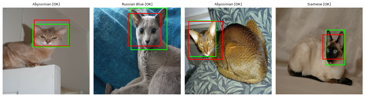
The clean baseline lands at breed accuracy ≈ 0.93, head-box IoU ≈ 0.67 — that’s the model everything downstream gets compressed from.

---

Part 2 — Pruning: remove what doesn’t matter

Why pruning works at all

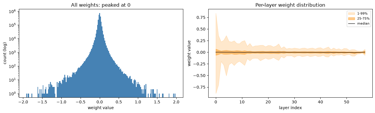
Plot the weight distribution of a trained network and you see the same thing every time: a dense spike at zero. Most weights are tiny, and a weight of 0.01 contributes almost nothing next to a weight of 0.8. That’s the slack pruning exploits.

Two distinctions that organize everything

• Unstructured vs structured. Unstructured removes individual weights (scored by magnitude, |w|); structured removes whole channels (scored by the L2 norm of the filter — a single weight isn’t the right unit when you delete the whole thing).
• Masking vs physical removal. Masking zeros weights in place — the tensor keeps its shape. Physical removal actually shrinks the tensor. This distinction is where most of the surprises live.

The trade-off falls straight out of those two axes. Unstructured keeps accuracy best but buys no speedup — the tensor is still dense, so ordinary kernels do the same work; the file only shrinks if you apply a sparse format (CSR) or gzip. Structured channel removal produces a smaller dense tensor that any hardware runs faster, at a bigger accuracy hit.

The math behind it

Importance scoring depends on the unit being removed — the magnitude of a single weight, or the L2 norm of a whole filter (a single weight isn’t the right unit when you delete the channel):

$$\text{score}_{\text{unstructured}} = |w|, \qquad \text{score}_{\text{channel}} = \lVert \mathbf{w}_f \rVert_2 = \sqrt{\sum_i w_i^2}$$

And here’s why structured pruning moves latency, not just size: a conv layer’s parameter count and FLOPs both scale linearly with channel count, so dropping channels cuts both at once.

$$\text{params} = C_{\text{in}}\, C_{\text{out}}\, k^2, \qquad \text{FLOPs} = H\, W\, C_{\text{in}}\, C_{\text{out}}\, k^2, \qquad \text{sparsity} = \frac{\#\{\, w = 0 \,\}}{\#\{\, w \,\}}$$

Remove an output channel and you delete a slice of $C_{\text{out}}$ in this layer and the matching $C_{\text{in}}$ in the next — fewer params and fewer FLOPs, on ordinary hardware.

The cliff, and the fragile head

Pruning everything at once (“one-shot”) with no recovery walks the model straight off a cliff — and notice which curve falls first:

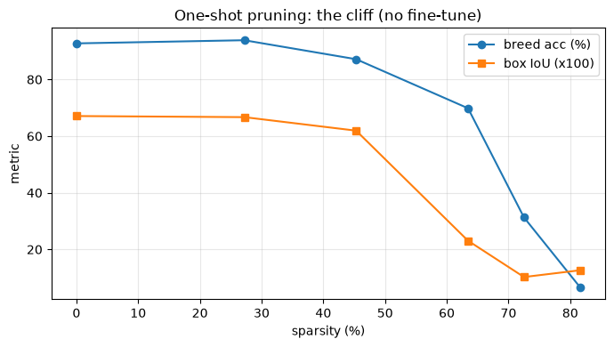
The box head is fragile: its IoU craters well before breed accuracy does. The practical consequence is that I excluded the box head from every pruner — protecting the task that breaks first. The fix for the cliff itself is to prune iteratively: remove a slice, fine-tune to recover, repeat. And the reason iterative beats one-shot is not simply “because it fine-tunes” (one-shot can fine-tune too) — it’s that (1) small increments stay recoverable, and (2) importance is re-estimated each round after the surviving weights redistribute, so you always cut the currently weakest weights instead of a stale ranking.

The dependency-graph problem (and the experiment that nails it)

Channel pruning has a catch that weight pruning doesn’t: layers are coupled. Removing an output channel of layer L deletes a feature map, which forces matching removals downstream — the corresponding input-channel slice of layer L+1, that channel’s BatchNorm parameters, and, in a ResNet, the residual add, whose two operands must keep equal channel counts. This isn’t an accident to avoid; it’s a consistency requirement. Tools like torch_pruning build a dependency graph (by tracing an example input) to propagate every removal so the network stays valid. (Don’t confuse this with “global pruning,” which is a separate idea — ranking importance across the whole model rather than per-layer.)

import torch.nn.utils.prune as prune   # masking: zeros in place, shape unchanged
import torch_pruning as tp             # physical removal via a dependency graph

# (A) Unstructured — rank all weights by |w| (L1), zero the smallest. A MASK.
prune.global_unstructured(prunable, prune.L1Unstructured, amount=0.3)

# (B) Structured — score each conv filter by its L2 norm (n=2) over the output dim, zero channels.
prune.ln_structured(conv, 'weight', amount=0.3, n=2, dim=0)

# (C) Physical channel removal — torch_pruning traces an EXAMPLE INPUT to build the dependency
#     graph, then actually shrinks the tensors (params drop -> smaller AND faster on ordinary HW).
ex = torch.randn(1, 3, 224, 224, device=DEVICE)
pruner = tp.pruner.MagnitudePruner(
    model, ex, importance=tp.importance.MagnitudeImportance(p=2),
    pruning_ratio=0.15, iterative_steps=3, ignored_layers=[model.cls_head, *model.box_head])
for _ in range(3):
    pruner.step()                      # remove channels this round
    finetune(model)                    # ...then recover

That prune.* path only writes a weight_mask, so even after you “bake” it the tensor shape — and the file size — is unchanged. torch_pruning rebuilds smaller tensors. The numbers make the distinction concrete:

Approach	Params	Raw / gzip	Sparsity	Acc / IoU
baseline	26.0M	104M / 97M	0%	0.927 / 0.671
unstructured (iterative)	26.0M	104M / 40M	69%	0.933 / 0.686
structured masked (no fine-tune)	26.0M	104M / 73M	27%	0.078 / 0.044
channel — iterative (physical removal)	19.3M	78M / 72M	0%	0.905 / 0.685

Two lessons jump out of that table. Unstructured at 69% sparsity gzips to 40 MB but the raw file is still 104 MB — masking is a compression story, not a smaller-tensor story. And structured masking without fine-tuning is the worst of all worlds: accuracy in the gutter (0.078!) and no size or speed win, because the tensor never actually shrank. Only physical channel removal gives a genuinely smaller model (26.0M → 19.3M params, 104 MB → 78 MB) that holds accuracy. That’s the one I carried forward.

---

Part 3 — Quantization: fewer bits per weight

Quantization maps a real value $r$ (a weight or activation) to a $b$-bit integer $q$ through an affine transform — a shared scale $S$ and an integer zero-point $Z$ — and dequantizes by inverting it:

$$q = \operatorname{clamp}\!\Big(\operatorname{round}\!\big(\tfrac{r}{S}\big) + Z,\; q_{\min},\, q_{\max}\Big), \qquad \hat{r} = (q - Z)\,S$$

For a $b$-bit signed integer the range and the parameters that fit a tensor with values in $[\,r_{\min}, r_{\max}\,]$ are

$$q_{\min} = -2^{\,b-1}, \quad q_{\max} = 2^{\,b-1}-1, \qquad S = \frac{r_{\max} - r_{\min}}{q_{\max} - q_{\min}}, \qquad Z = \operatorname{round}\!\Big(q_{\min} - \frac{r_{\min}}{S}\Big)$$

The symmetric int8 case I actually used is just this with the offset dropped ($Z = 0$), a zero-centered range ($r_{\max} = \max(|r|)$), and $b = 8$ — which collapses the scale to the familiar $S = \max(|r|)\,/\,127$. Drop to $b = 4$ and the same formulas give int4.

A few more facts worth knowing cold:

• int8 × int8 accumulates in int32 to avoid overflow, then requantizes back to int8.
• Per-tensor uses one scale for the whole tensor; per-channel uses one per output channel — more accurate, and the default for conv weights.

The variants differ by what gets quantized and when the activation ranges are decided:

• Weight-only: weights int8 (size win), dequantized to FP32 for a float matmul. Size only.
• Dynamic: weights int8; activation ranges computed at runtime, per op. In PyTorch this only has kernels for Linear/LSTM — there’s no dynamic Conv — so on a conv-heavy ResNet it barely does anything (below, it shrinks the model by 1.1×).
• Static: weights and activations int8, with activation ranges fixed offline by a calibration pass over representative data. Weights don’t need calibration data — only activations do, since you can’t know their ranges without running the model.
• QAT (Quantization-Aware Training): insert fake-quant ops (quantize-then-dequantize) on weights and activations during fine-tuning so the network learns to tolerate int8 rounding. The forward pass stays FP32 because the rounding is non-differentiable — you backprop through it with the straight-through estimator. At export the fake-quant is replaced by real int8 ops (keeping the learned scales), and the deployed activations flow as int8 with an FP32 output at the boundary.

All four are a handful of lines on top of the pruned FP32 model. The thing to read off the code is how much machinery each one needs — weight-only is a tensor rewrite, static needs a calibration loop, QAT needs an actual training loop:

import copy, torch, torch.nn as nn
torch.backends.quantized.engine = 'qnnpack'   # ARM / Apple Silicon int8 backend; quantized ops are CPU-only
example_inputs = (torch.randn(1, 3, 224, 224),)

# (A) Weight-only — round each conv/linear weight to int8 with a PER-OUTPUT-CHANNEL scale (S = max|w|/127),
#     activations stay FP32. No data, no training. Here we fake it (quantize->dequantize) to read the accuracy hit.
def fake_weight_int8(m):
    mc = copy.deepcopy(m)
    for mod in mc.modules():
        if isinstance(mod, (nn.Conv2d, nn.Linear)):
            w = mod.weight.detach(); dims = tuple(range(1, w.dim()))     # reduce over all but the output dim
            scale = (w.abs().amax(dim=dims, keepdim=True) / 127).clamp(min=1e-8)
            mod.weight.data = torch.round(w / scale).clamp(-127, 127) * scale
    return mc

# (B) Dynamic — weights int8, activation ranges picked at runtime. Only has Linear/LSTM kernels, so on a
#     conv-heavy ResNet it touches just the head Linears -> barely shrinks (the 1.1x row).
from torch.ao.quantization import quantize_dynamic
md = quantize_dynamic(copy.deepcopy(fp32), {nn.Linear}, dtype=torch.qint8)

# (C) Static — weights AND activations int8. prepare_fx inserts OBSERVERS; calibration runs representative
#     data to fix activation ranges (weights need none); convert_fx swaps in real int8 ops. FX auto-fuses conv-bn-relu.
from torch.ao.quantization import quantize_fx, get_default_qconfig_mapping
prepared = quantize_fx.prepare_fx(copy.deepcopy(fp32).eval(), get_default_qconfig_mapping('qnnpack'), example_inputs)
with torch.no_grad():
    for i, (x, _, _) in enumerate(calib_loader):   # a few hundred images is plenty
        prepared(x)
        if i >= 7: break
static_int8 = quantize_fx.convert_fx(prepared)

# (D) QAT — prepare_qat_fx inserts FAKE-QUANT (quant->dequant, FP32 forward, straight-through backward) so the
#     net LEARNS to tolerate int8. Fine-tune from the pruned weights, then convert to real int8 ops.
from torch.ao.quantization import get_default_qat_qconfig_mapping
qat = quantize_fx.prepare_qat_fx(copy.deepcopy(fp32).train(), get_default_qat_qconfig_mapping('qnnpack'), example_inputs)
opt = torch.optim.AdamW(qat.parameters(), lr=1e-5, weight_decay=1e-4)
for _ in range(QAT_EPOCHS):
    run_epoch_mt(qat, train_loader, 'cpu', opt, lam=LAMBDA)   # ordinary training loop, just with fake-quant in the graph
qat_int8 = quantize_fx.convert_fx(qat.eval())

Technique	Size	× smaller	Acc / IoU
FP32 (pruned baseline)	78 MB	1.0×	0.905 / 0.685
weight-only	20 MB	3.9×	0.905 / 0.685
dynamic	73 MB	1.1×	0.905 / 0.685
static	19 MB	4.0×	0.883 / 0.683
QAT	19 MB	4.0×	0.872 / 0.677

The decision rule: try static PTQ first; escalate to QAT only if the accuracy drop is too big. And there’s that dynamic row — 1.1×, basically free of effect — exactly because a ResNet is almost all conv and dynamic quant only touches Linear. Right conclusion (dynamic is the wrong tool for a CNN), for the precise reason (kernel coverage, not “overhead”).

---

The ship decision

Putting every variant on one chart — predicted vs ground-truth boxes, all models, one figure — is the honest way to choose:

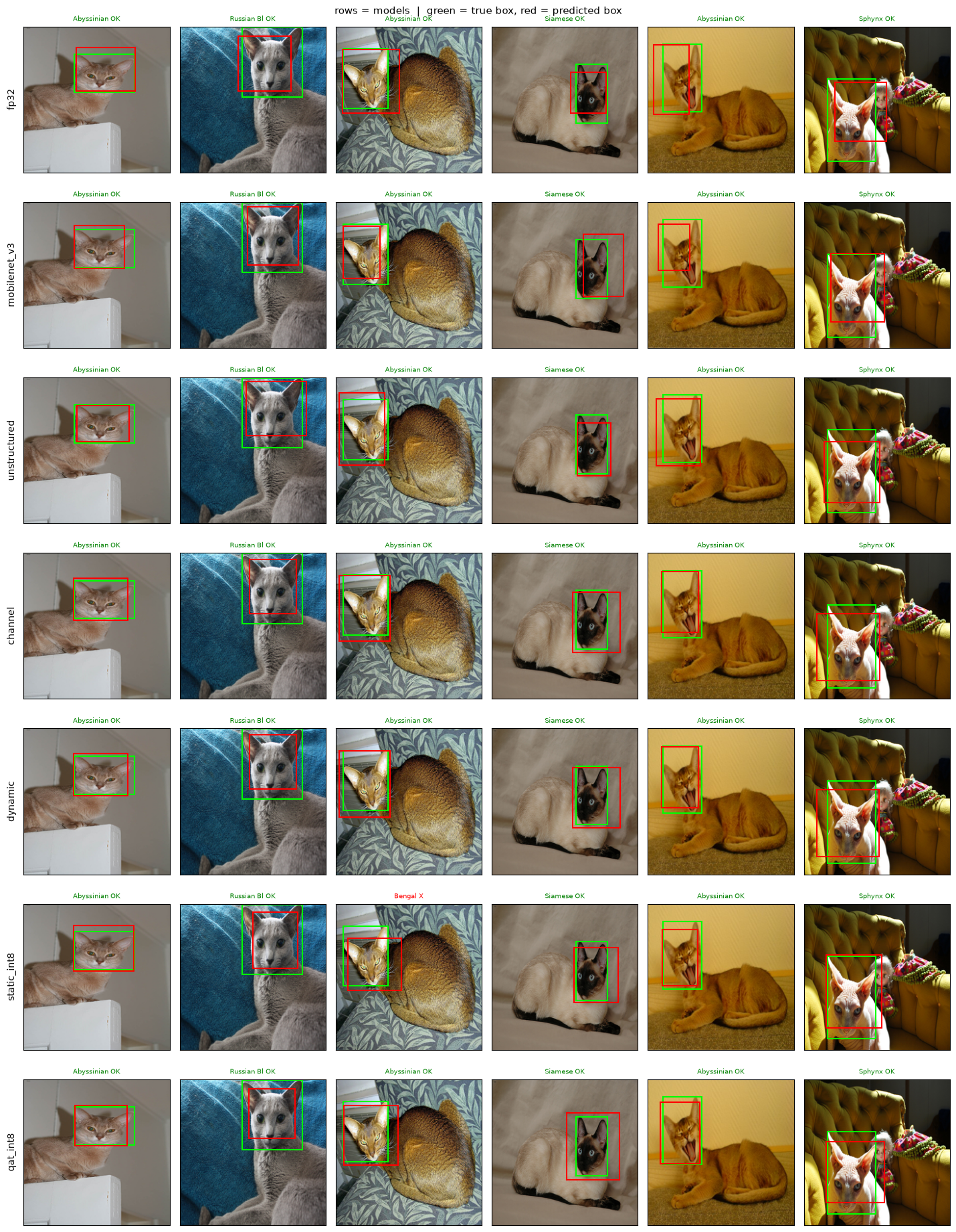
So which would I ship? It depends on the axis you’re optimizing:

• For this learning project, the channel-pruned + int8 ResNet is the satisfying answer — 19 MB at ~0.90 breed accuracy, a clean 5× size cut from the 104 MB baseline with the full compression story behind it.
• For an actual product, the honest answer is MobileNetV3 — 15 MB at the same ~0.90 accuracy, with far fewer params and FLOPs. A backbone designed for the edge beats a heavyweight-then-compressed one. The compression pipeline taught me far more; the native-edge model would win the ship review. Naming that tension out loud is the point.

---

What I’d actually keep (the transferable lessons)

• Name the axis. Every technique moves size, latency, or accuracy — say which. Quantization cuts bytes and per-op cost, not FLOP count; structured pruning cuts FLOPs.
• Masking ≠ removal. Sparsity is a compression win; a smaller dense tensor is the speed win. A 69%-sparse masked model is still 104 MB.
• Use the spatial map for the spatial task. Global average pooling destroys location — fine for classification, fatal for a bounding box.
• Protect the fragile head. The box regressor breaks before the classifier; exclude it from pruning.
• Iterative beats one-shot because of small recoverable steps and re-estimated importance — not merely because it fine-tunes.

The corrections were the curriculum. Every number in this post came from a notebook run, including the ones that embarrassed an earlier draft of my own understanding — which is exactly why I wrote them down.