96% full-board accuracy on chess recognition — what the papers say and what actually worked
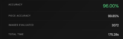
This was built for an online chess-recognition challenge: given rendered chessboard images from a held-out test set, predict the FEN string for each position. The evaluator scores two things — per-square accuracy and full-board accuracy — and returns results in real time. Here is what the submission page showed:
| Metric | Result |
|---|---|
| Per-square accuracy (val) | 99.85% |
| Full-board accuracy (val) | 96% |
| Inference latency (GPU FP16) | ~40 ms |
| Inference latency (CPU) | ~500 ms |
| Training epochs | 30 |
| Dataset size | 12,252 train / 3,072 test |
96% full-board means roughly 96 out of 100 boards have every single square correct — one wrong square fails the whole board. The per-square rate (99.85%) puts the per-cell error at about 1.5 in 1,000. This post is a walkthrough of every design decision that got there, with the paper that justified each one.
The problem: pixels in, FEN string out
The task: given one top-down rendered PNG of a chessboard, predict the FEN piece-position string.
What is FEN? FEN (Forsyth–Edwards Notation) is a compact way to describe where every piece sits on a chessboard. A string like rnbqkbnr/pppppppp/8/8/2P5/8/PP1PPPPP/RNBQKBNR encodes all 64 squares — uppercase for white pieces, lowercase for black, digits for runs of empty squares. One FEN string = one complete board position.
There are 13 possible classes per square: empty, plus the 12 piece types (K Q R B N P in upper and lower case).

Why is full-board accuracy the right metric? A model that is 99% per-square accurate but consistently wrong on one square per board scores 0% full-board. Every square must be correct for the board to be usable. Per-square accuracy is a training signal; full-board accuracy is the real-world score.
The full pipeline at a glance
What the papers said before writing a line of code
My principle going in: every component must have a paper behind it, or I need my own ablation experiment to justify it. That kept me from chasing intuitions.
| Paper | Year | Key result | Role in this project |
|---|---|---|---|
| CVChess (Abeykoon et al.) | 2025 | 98.93% per-square on real photos | Architecture blueprint |
| ResNet (He et al.) | 2015 | Residual connections enable 50+ layer training | Backbone |
| ImageNet (Russakovsky et al.) | 2015 | 1.3M labeled images for pretraining | Pretrained weights |
| LiveChess2FEN (Mallasén Quintana et al.) | 2020 | 92% per-piece + legality Algorithm 2 | Post-processing rules |
| Neural Chessboard (Czyzewski et al.) | 2017 | ~95% per-piece + chess rule enumeration | Hard chess constraints |
| Chesscog (Wölflein & Arandjelović) | 2021 | 99.77% per-square on synthetic data | Accuracy baseline |
| End-to-End (Masouris & van Gemert) | 2024 | DETR “failed to converge” | Negative result — ruled out Transformers |
Architecture blueprint — CVChess (Abeykoon et al., 2025)
CVChess is the direct blueprint for the model architecture. The paper proposes a pipeline: ResNet-50 backbone → AdaptiveAvgPool(8, 8) → reshape to (64, 2048) → Linear(2048 → 13). They report 98.93% per-square accuracy on real photographs — a significantly harder domain than rendered images. If this architecture handles real photos at 98.9%, it should handle clean synthetic renders well above that.
The key insight CVChess demonstrates is per-square classification with a shared head. One linear layer predicts all 64 squares simultaneously, sharing the same weights.
Why shared weights instead of 64 separate classifiers? A white king looks the same whether it stands on e1 or d4. You want the same detector to fire wherever a white king appears, regardless of which square it occupies. Shared weights enforce that — the model learns “what a white king looks like” once, not 64 times. This uses 2,048 × 13 = 26,624 parameters instead of 64 times as many.
I adopted CVChess’s architecture verbatim, adding only ImageNet pretrained weights and horizontal flip augmentation.
Backbone — ResNet (He et al., 2015)
What is a residual network? Before 2015, adding more layers to a neural network reliably made it train worse, not better. The problem is vanishing gradients: during backpropagation, the error signal multiplies through dozens of weight matrices on its way to the early layers, shrinking exponentially until the gradient is nearly zero. Early layers stop learning.
ResNet’s fix is a shortcut connection. Instead of output = F(x), a residual block computes output = F(x) + x. The plain input is added back to the block’s output. This gives gradients an express lane to early layers — instead of multiplying through every weight matrix, they can flow directly through the addition. He et al. showed that a 152-layer network could train reliably with this trick, and their CVPR 2016 Best Paper award reflects how transformative it was.
Why pretrained on ImageNet? Russakovsky et al. (2015) created ImageNet: 1.3 million labeled photographs across 1,000 categories. A ResNet-50 trained on ImageNet has already learned to detect edges, textures, gradients, and shapes from natural images. Fine-tuning from this starting point costs a fraction of training from scratch — the early layers already know how to look at images. We load these weights via torchvision.models.ResNet50_Weights.IMAGENET1K_V2.
Legality post-processing — LiveChess2FEN (Mallasén Quintana et al., 2020)
LiveChess2FEN runs on a Jetson Nano for real-time physical board recognition, reporting 92% per-piece accuracy and 95% board detection. Their contribution relevant here is a fixed-point legality post-processor (Algorithm 2) that applies hard chess rules after inference:
- R1: each side has exactly one king — if the model predicts two, demote the lower-confidence one
- R2: pawns cannot appear on the back rank (row 1 or row 8)
- R3: piece count limits — each side has at most 8 pawns, 2 rooks, 2 bishops, 2 knights, 1 queen
Why post-process instead of adding these rules to the loss function? Hard count constraints in a loss function create conflicting gradients. If the model predicts two white kings, the loss term that penalizes this fires on both squares simultaneously, pushing each square’s prediction in opposite directions. Training becomes unstable. Post-processing with confidence-based demotion is cleaner: after inference, if two white kings appear, keep the square with higher softmax probability and replace the other with its second-most-likely class. The model’s own confidence distribution makes the call.
I implemented Algorithm 2 directly in chess_recognition/legality.py.
Hard chess rule set — Czyzewski et al. (2017)
Czyzewski et al. report ~95% per-piece accuracy and 99.57% lattice point detection. Their contribution relevant here is the enumeration of hard chess constraints, which I used to populate the R3 piece count rules above.
Why not a Transformer? — Masouris & van Gemert (2024)
Masouris and van Gemert tried a DETR variant (a Transformer-based object detection architecture) for chess recognition and reported it “failed to converge”.
Why is this a valuable result? DETR was designed to detect a variable number of objects at unknown locations. A chessboard is the opposite problem: exactly 64 predetermined locations, no need to find anything. The per-square CNN classification approach from CVChess is the right inductive bias for a fixed grid. DETR’s flexibility is a liability when your output space is fully rigid. This negative result saved several days of investigation.
Synthetic images are tractable — Chesscog (Wölflein & Arandjelović, 2021)
Chesscog achieves 99.77% per-square accuracy on synthetic data, confirming that CNNs can classify rendered chess pieces to high accuracy. I did not use their board detection pipeline because in this dataset the camera is fixed — but their accuracy number set the expectation for what was achievable.
The key insight from EDA: the camera does not move
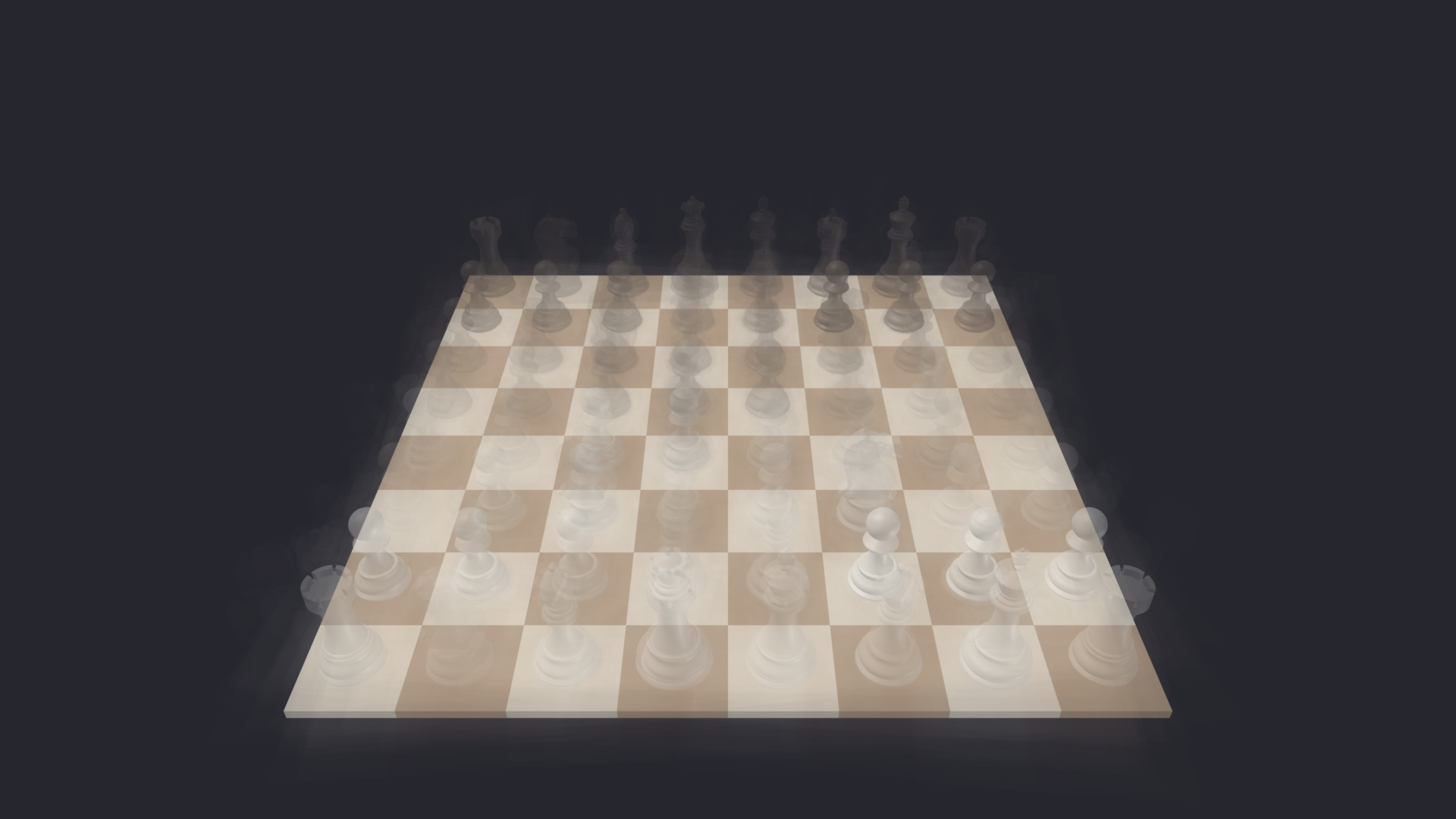
Before building the model, I averaged 200 training images pixel-by-pixel. If the camera moves between shots, the average blurs everywhere. If the camera is fixed, the static parts (the board surface) stay sharp while the moving parts (the pieces) blur out.
The average image showed a crystal-clear board outline and completely blurred pieces. One observation, two architectural decisions:
1. Cached homography. A homography is a 3×3 matrix that maps points on a tilted plane to a flat top-down view. cv2.getPerspectiveTransform computes the matrix from the four board corners, mapping the board to a 512×512 canonical view where each square occupies exactly 64×64 pixels. Because the camera never moves, compute this matrix once and reuse it for every image.
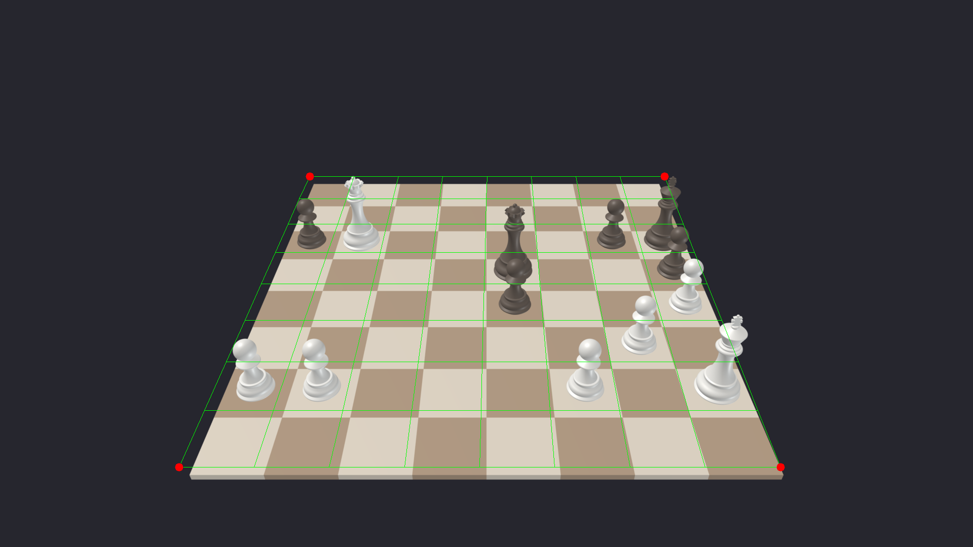
cv2.getPerspectiveTransform. The green grid shows the resulting 8×8 projection — each cell maps to exactly one chess square in the warped 512×512 image. This matrix is computed once and cached for all subsequent frames.Chesscog needed a full detection pipeline for board localization. This project skips it entirely — the cached homography does the job in microseconds.
2. Hash-based insurance. Compute a SHA-256 hash of the top strip of the image (rows y=0..300, which shows only the background — no pieces). Same hash → camera in same position → use cached matrix. Different hash → camera moved → fall back to classical edge detection. Pieces occupy y=348 and below, so the hash is never influenced by piece positions.
The piece misalignment problem (and why full-board classification solves it)
Homography corrects the board surface — a flat 2D plane. Chess pieces are 3D objects. After warping, a tall piece like the king has its base (the ground truth label location) in square e4, but its crown can project into e5 or beyond.
The naive approach fails. Cropping 64 individual squares and running 64 separate classifiers makes this unsolvable: the most distinctive pixels for identifying the king in its square might be sitting in the adjacent square’s crop.
The CVChess solution. Classify all 64 squares from the full 512×512 image in one forward pass. ResNet-50 with a 32× stride has a receptive field of roughly 483×483 pixels at the deepest layers — nearly the full image. Each feature cell encodes context from a large patch of the board, not just one square.
Analogy: imagine a panel of judges assessing 64 candidates simultaneously by watching them all work in the same room, rather than calling each one into a separate booth. The panel can see that the person labeled as sitting in seat 12 is actually reaching into seat 13 — because they have the full-room view. The per-booth interviewer would just see an empty seat.
Architecture: from pixels to FEN
The full inference pipeline with actual tensor shapes at each step:
Input:  PNG  →  1080 × 1920 × 3    (H × W × BGR uint8)
         ↓
BGR→RGB + cv2.warpPerspective
         ↓
Warped: 512 × 512 × 3              (1 square = 64×64 px)
         ↓
Normalize (/255, ImageNet mean/std)
         ↓
Tensor: 1 × 3 × 512 × 512          (B, C, H, W float32)
         ↓
ResNet-50 (Layer 4 output)
         ↓
Features: 1 × 2048 × 16 × 16       (NOT pixels — feature cells)
         ↓
AdaptiveAvgPool(8, 8)
         ↓
Pooled: 1 × 2048 × 8 × 8           (1 cell = 1 chess square)
         ↓
Reshape → 1 × 64 × 2048
         ↓
Linear(2048 → 13)
         ↓
Logits: 1 × 64 × 13                (13 scores per square)
         ↓
Softmax + argmax + legality rules
         ↓
FEN string: "rnbqkbnr/pppppppp/..."
Understanding the three unit types
The 16×16 after ResNet-50’s layer 4 is not pixels. It is 16×16 feature cells, each holding 2048 channels of extracted features. One feature cell covers 32×32 pixels of the warped image. After pooling to 8×8, each cell covers 64×64 pixels — exactly one chess square.
The 2048 numbers per cell are not color values; they are learned representations of shapes, textures, and spatial relationships that ResNet extracted from that region.
Model parameters. ~23M in the ResNet-50 backbone; 26,624 in the linear head (2048 × 13).
Training: two-phase fine-tuning
Why two phases? When you attach a randomly initialized head to a pretrained backbone, the head produces large, noisy gradients early in training — it has no idea what to do yet. If the backbone is unfrozen from the start, those noisy gradients corrupt the ImageNet features the backbone already learned before the head has stabilized.
| Phase 1 (epochs 1–3) | Phase 2 (epochs 4–30) | |
|---|---|---|
| Backbone | Frozen — 23M params unchanged | Unfrozen — gently fine-tuned |
| Head LR | 1e-3 | 1e-3 |
| Backbone LR | N/A | 1e-4 |
| LR schedule | Constant | CosineAnnealingLR |
| Purpose | Align head to existing ImageNet features | Adapt backbone features to chess textures |
| Full-board acc. at end | 10.4% | 96% |
The effect of unfreezing is stark. At the end of epoch 3 (frozen), full-board accuracy was 10.4%. At the end of epoch 4 (first epoch unfrozen), it jumped to 62.9% — a 52-point gain from a single epoch of backbone fine-tuning.
Loss function: weighted cross-entropy. The dataset is imbalanced — roughly half of all squares are empty in any position. Without weighting, the model’s easiest path is to predict “empty” everywhere and score ~50% per-square accuracy while producing useless FENs. Inverse-frequency class weights (capped at 5× to prevent rare pieces like queens from dominating training) fix this by making mistakes on occupied squares more costly.
Augmentation. Horizontal flip with symmetric FEN label remapping (column a↔h, b↔g, etc. — a flipped board is still a valid board with mirrored piece positions), plus color jitter ±10% on brightness, contrast, and saturation.
Legality post-processing in practice
The neural network does not know chess rules. It has seen 12,252 boards during training and learned statistical patterns, but it is not guaranteed to output a legal board. In testing, the most common illegal predictions were:
- Two kings of the same color (model was close to 50/50 on a low-contrast square)
- A pawn on the back rank (class confusion between pawn and empty near the board edge)
The LiveChess2FEN fixed-point algorithm resolves these with confidence-based demotion. When the model predicts two white kings, keep the square with the highest softmax probability as king, and replace the other with its second-most-likely class. Iterate until no rules are violated.
In practice, this never ran more than 2 iterations on the validation set.
Results
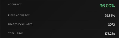
Training results from runs/v1/history.json:
| Epoch | Per-square (val) | Full-board (val) |
|---|---|---|
| 1 | 89.3% | 6.8% |
| 3 | 89.6% | 10.4% |
| 4 ✦ unfreeze | 96.0% | 62.9% (+52 pts in 1 epoch) |
| 10 | 99.3% | 83.0% |
| 17 | 99.6% | 90.3% |
| 25 | 99.8% | 95.0% |
| 30 (final) | 99.85% | 96.0% |
Why is full-board accuracy lower than per-square accuracy? The math explains the gap. If each square has an independent 0.15% error rate, the probability that all 64 are correct is 0.9985^64 ≈ 0.907, or about 90.7%. The actual 96% is better than this naive independence model — errors are not uniformly distributed across all boards and squares. The model gets most boards perfectly right and clusters its mistakes on a subset of hard positions. If errors were random, we’d expect ~91%; the actual 96% means the model has learned to handle most positions reliably.
Comparison. Chesscog (Wölflein & Arandjelović, 2021) reports 99.77% per-square on synthetic data with a more complex pipeline including separate board detection. This project reaches 99.85% with a simpler approach — no separate board detection, no per-square crop model, one unified forward pass.
What did not work
The Masouris & van Gemert (2024) DETR-based approach explicitly failed to converge, as documented in their paper. The structural reason: DETR is built to solve “how many objects are there, and where are they?” A chessboard has exactly 64 fixed locations — there is nothing to locate. The fixed-grid inductive bias of per-square CNN classification is simply the correct fit for this problem.
Summary of design decisions and their sources
| Decision | Justification | Source |
|---|---|---|
| ResNet-50 backbone | Residual connections enable deep training; ImageNet pretraining provides strong features | He et al. (2015) |
| Per-square Linear head | Shared weights, fixed-grid output — 98.93% on real photos | CVChess |
| 512×512 input | Divisibility by 32 (ResNet stride), alignment to 8×8 grid, memory budget | CVChess (adapted) |
| ImageNet pretrained weights | Match the backbone’s expected input distribution | Russakovsky et al. (2015) |
| Fixed-point legality rules | Stable post-processing without loss instability | LiveChess2FEN |
| Hard chess constraints (R1/R2/R3) | Enumerated rule set | Czyzewski et al. (2017) |
| No Transformer | DETR failed to converge on this task | Masouris & van Gemert (2024) |
| Cached homography | Camera fixed → compute once, reuse | EDA observation (this project) |
| Two-phase fine-tuning | Prevent head’s initial gradients from corrupting backbone | Standard practice, confirmed empirically |
| Weighted cross-entropy | ~50% empty squares cause class imbalance | Standard practice |
References
- Abeykoon et al. (2025). CVChess: A Robust Chess Recognition Pipeline. arXiv:2511.11522
- He, K., Zhang, X., Ren, S., & Sun, J. (2015). Deep Residual Learning for Image Recognition. arXiv:1512.03385. CVPR 2016 Best Paper.
- Mallasén Quintana et al. (2020). LiveChess2FEN: a Framework for Classifying Chess Pieces based on CNNs. arXiv:2012.06858
- Czyzewski et al. (2017). Neural Chessboard. arXiv:1708.03898
- Russakovsky et al. (2015). ImageNet Large Scale Visual Recognition Challenge. arXiv:1409.0575
- Wölflein, G. & Arandjelović, O. (2021). Recognizing Chessboards and Their Pieces in the Wild. arXiv:2103.07919
- Masouris, A. & van Gemert, J. (2024). End-to-End Chess Recognition. arXiv:2310.04086