What continuous batching changes: reading three LLM inference traces
I wanted to see what batching changes inside an inference loop, rather than stop at benchmark numbers. I implemented three schedulers around the same Qwen model and recorded their model calls with PyTorch Profiler:
- Serial inference processes one request from prefill through decode.
- Static batching creates a closed group and runs it until every member finishes.
- Continuous batching can change membership after every model iteration.
The result can be summarized in one causal chain:
scheduling policy
→ batch membership over time
→ number and shape of model calls
→ queueing and work completed per call
→ throughput and tail latency
Continuous batching performed best in this experiment because it kept more requests making progress together. Throughput, TTFT, and E2E latency are different measurements of that same underlying scheduling behaviour, so I analyze them together rather than as three independent findings.
The controlled workload
All three schedulers processed the same burst:
| Setting | Value |
|---|---|
| Model | Qwen2.5-1.5B-Instruct |
| Device | PyTorch MPS |
| Concurrent requests | 16 |
| Maximum active batch size | 8 |
| Output-length pattern | 4, 16, 8, 12, repeated four times |
| Total output tokens | 160 |
| Continuous token budget | 256 per iteration |
| Maximum prefill chunk | 64 tokens per request |
The mixed output lengths are intentional. Within each group of eight, two requests need 4 tokens, two need 8, two need 12, and two need 16. Short requests therefore retire before long ones, exposing the difference between a closed static batch and an iteration-level continuous batch.
Each strategy ran in a fresh server process and warmed up before recording. These are profiled timings from one experiment, not clean production benchmarks.
The result in one table
| Strategy | Model calls | Model-step span | Output tok/s | TTFT p95 | E2E p95 |
|---|---|---|---|---|---|
| Serial | 160 | 4.158 s | 38.44 | 3893.8 ms | 4160.0 ms |
| Static batching | 32 | 2.359 s | 67.57 | 1224.6 ms | 2366.5 ms |
| Continuous batching | 29 | 1.270 s | 125.57 | 783.5 ms | 1272.5 ms |
The three strategies generated exactly the same 160 output tokens. Batching did not remove output work; it allowed one model call to advance multiple requests.
| Strategy | Output tokens per model call |
|---|---|
| Serial | 1.00 |
| Static | 5.00 |
| Continuous | 5.52 |
Call count alone is not a performance metric—a larger batched call can take longer than a batch-one call. Here, the trace shows both fewer calls and more useful work inside them, while the elapsed-time measurements show that the grouping paid off.
Serial: 160 tokens became 160 sequential calls
The serial trace contained only:
miniserve.serial.prefill batch=1
miniserve.serial.decode batch=1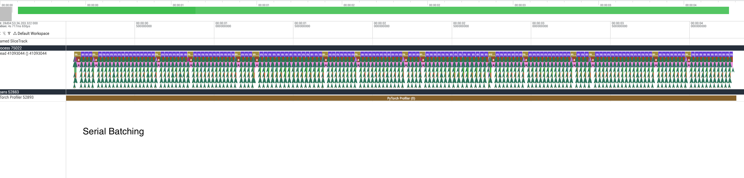
Prefill processes one request’s prompt and produces its first output token. Every later decode call produces one more token for that same request. For a request asking for (N) output tokens, this implementation therefore performs:
1 prefill call + (N - 1) decode calls = N model callsThe output pattern sums to 40 tokens and repeats four times:
(4 + 16 + 8 + 12) × 4 = 160That produced 16 prefill calls and 144 decode calls. Although the clients submitted 16 requests concurrently, the scheduler handled one request to completion before moving to the next. Later requests spent most of their TTFT waiting behind earlier requests; the model did not spend 3.9 seconds computing one first token.
Static batching: fewer calls, but a shrinking closed batch
Sixteen requests and a maximum batch size of eight created two closed batches. Each batch needed one prefill call followed by 15 decode iterations, because its longest requests required 16 output tokens:
2 closed batches × (1 prefill + 15 decode) = 32 model callsThe trace for each batch followed this shape:
prefill batch=8

3 × decode batch=8  → the 4-token requests finish
4 × decode batch=6  → the 8-token requests finish
4 × decode batch=4  → the 12-token requests finish
4 × decode batch=2  → the 16-token requests finish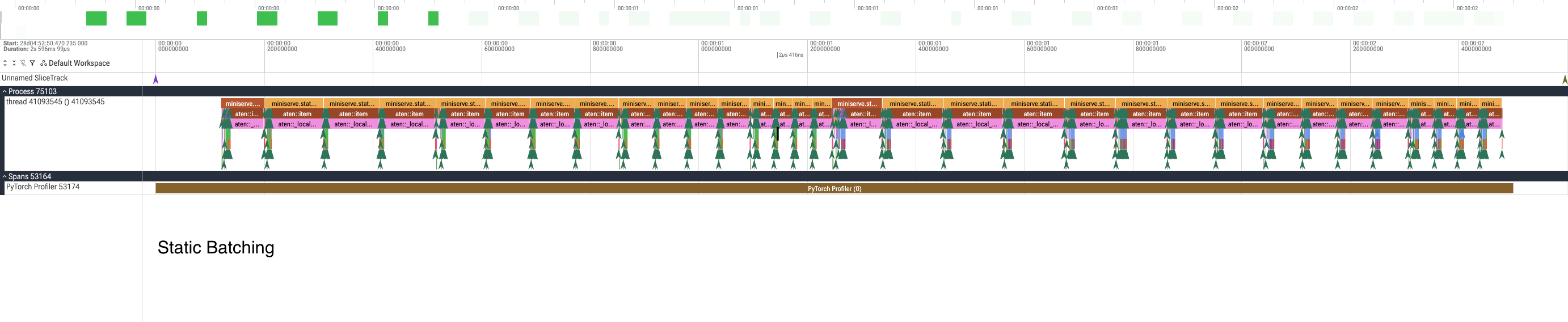
During the first batch, eight requests were still waiting. The scheduler could not place them into the six, four, and then two empty positions because static membership remained closed until the longest members finished.
Approximately 65% of static model-call busy time was spent below the maximum batch size. A smaller batch made an individual forward call shorter, but it also produced fewer output tokens:
| Static decode size | Average call duration | Output tokens per call |
|---|---|---|
| 8 | 108.3 ms | 8 |
| 6 | 87.7 ms | 6 |
| 4 | 63.3 ms | 4 |
| 2 | 40.2 ms | 2 |
The inefficiency is not that a batch=2 call is slow by itself. It is that the
call leaves six available sequence positions unused while work is waiting.
Continuous batching: refill between iterations
Continuous batching uses a logical ragged batch. The scheduler first assigns one token to every decoding request, then spends the remaining iteration budget on bounded prefill chunks. The backend packs those scheduled tokens into one tensor, supplies per-request positions and KV-cache ranges, and uses an isolating attention mask for one model forward pass.
A trace label describes that plan:
active=8 decode=5 prefill=3 tokens=44It means eight requests participated: five advanced by one decode token and
three contributed prompt chunks. tokens=44 is the total number of scheduled
query tokens, not the number of requests or generated outputs.
The trace showed the refill process directly:
active=8 decode=1 prefill=7 tokens=85
active=8 decode=5 prefill=3 tokens=44
active=8 decode=7 prefill=1 tokens=19
active=8 decode=8 prefill=0 tokens=8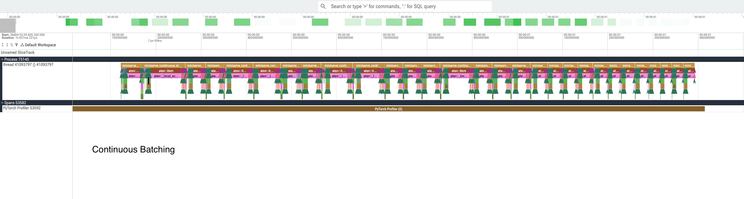
After each forward pass, completed requests were retired. Before the next iteration, requests from the waiting queue entered the newly available slots. Existing requests could therefore continue decoding while newly admitted requests performed prefill.
The active set stayed at eight through the central part of the workload. It only fell to seven, five, two, and one after the waiting queue was empty and no work remained to refill the tail.
Occupancy explains the benchmark together
| Occupancy observation | Static | Continuous |
|---|---|---|
| Model-call busy time at maximum active size | 35.0% | 64.5% |
| Model-call busy time below maximum | 65.0% | 35.5% |
How I calculated these occupancy percentages (Click to expand)
The denominator is the sum of the dur field for every miniserve.*
model-call event. It excludes the small gaps between calls. “At maximum” sums
events labelled batch=8 for static batching or active=8 for continuous
batching:
time-weighted maximum occupancy
= busy time at active size 8 / total model-call busy time
For static batching, the trace durations were:
| Active size | Calls | Busy time |
|---|---|---|
| 8 | 8 | 821.662 ms |
| 6 | 8 | 701.270 ms |
| 4 | 8 | 506.252 ms |
| 2 | 8 | 321.831 ms |
| Total | 32 | 2351.015 ms |
at maximum   = 821.662 / 2351.015 = 34.95% ≈ 35.0%
below maximum = (701.270 + 506.252 + 321.831) / 2351.015
              = 65.05% ≈ 65.0%
For continuous batching:
| Active size | Calls | Busy time |
|---|---|---|
| 8 | 15 | 813.601 ms |
| 7 | 1 | 43.089 ms |
| 5 | 4 | 137.168 ms |
| 2 | 4 | 122.567 ms |
| 1 | 5 | 144.621 ms |
| Total | 29 | 1261.045 ms |
at maximum   = 813.601 / 1261.045 = 64.52% ≈ 64.5%
below maximum = (43.089 + 137.168 + 122.567 + 144.621) / 1261.045
              = 35.48% ≈ 35.5%
This is duration-weighted logical request occupancy, not physical GPU utilization.
This difference connects the trace to all three headline metrics:
- Throughput: more requests advanced per model call, so continuous batching produced 125.57 output tok/s versus 67.57 for static and 38.44 for serial.
- TTFT: waiting requests could enter active execution before every older request completed, reducing queueing behind long generations.
- E2E latency: more requests made progress during the same model iterations, so the complete 16-request workload retired sooner.
These are not three unrelated wins. Dynamic membership reduced idle batching capacity and queueing; higher throughput and lower tail latency were two consequences of that decision.
The continuous trace contained 29 model steps over 1.270 seconds. Their model regions accounted for 1.261 seconds, with only about 9 milliseconds of gaps between them. At the CPU scheduling level, the worker was supplied with work almost continuously.
What this trace does—and does not—prove
The trace provides direct evidence of:
- one-request serial execution;
- static batch shrinkage without refill;
- mixed prefill and decode in continuous iterations;
- changing logical membership between continuous iterations;
- model-call count, duration, and CPU-side scheduling gaps.
It does not prove GPU saturation. On MPS, this PyTorch trace shows logical
model regions and CPU-side operator dispatch, not Metal kernel activity. An
active=8 decode step processes eight query tokens, while an active=8
prefill-heavy step may process many more. Active request count is therefore a
measure of scheduling occupancy, not a GPU utilization percentage.
The profiled run also adds overhead, uses one model and one machine, and was captured once with a workload deliberately chosen to expose length variation. Repeated non-profiled runs are required before treating the timing ratios as general performance claims.
Key takeaways
- Concurrency is not batch size. Sixteen requests can be in the system while only eight are active in a model iteration.
- Batching does not reduce requested output tokens. It increases the useful work completed per model call.
- Static batching wastes the holes created by short requests. It cannot refill until the entire closed batch retires.
- Continuous batching refills between iterations. It can combine old decode work with new prefill work in the next packed forward pass.
- Throughput and tail latency share a cause here. Better batch occupancy lets more requests progress and spend less time waiting.
- A scheduler trace is not a GPU utilization trace. It explains the shape of submitted model work; hardware counters are needed to identify actual accelerator saturation.