Where does LLM inference time go? Prefill, decode, and KV cache on Apple silicon

Calling model.generate() makes text generation look like one operation. It is not. Underneath it is a stateful loop with two phases that place very different demands on the hardware:

• Prefill processes the whole prompt in parallel, creates the key-value (KV) cache, and produces the first output token.
• Decode processes one new token at a time, reuses the cache, and extends it until generation stops.

I wanted to understand that loop well enough to implement it myself—not merely memorize the PyTorch syntax. I then profiled one generation on an Apple M4 Pro through both PyTorch and Apple’s Metal tools.

The experiment left me with four main conclusions:

1. Prefill presents much denser GPU work because many prompt tokens can be processed together.
2. Batch-one decode presents short, repeated GPU bursts because its token dependency makes the loop sequential.
3. KV caching removes repeated computation, but its storage grows linearly with sequence length.
4. Apple silicon’s unified memory removes the traditional system-RAM-to-VRAM copy boundary; it does not remove caches, synchronization, bandwidth limits, or data movement.

This report develops those conclusions from the code and measurements, then compares the PyTorch MPS/Metal path with CUDA on an NVIDIA GPU.

---

The experiment

I deliberately owned the generation loop instead of calling model.generate().

Component	Setup
Machine	MacBook Pro, Apple M4 Pro, 48 GB unified memory
Model	Qwen2.5-1.5B-Instruct
Backend	PyTorch mps
Precision	FP16
Batch size	1
Prompt	512 tokens
Output	32 new tokens, greedy decoding
Warm-up	3 generations before capture
Profilers	PyTorch Profiler/Perfetto and Instruments/Metal Debugger

This is a profiling study, not a CUDA-versus-MPS performance benchmark. Profiler overhead means the captured timings should not be mixed with clean latency measurements.

The generation loop I implemented

The engine returns explicit result objects rather than an unstructured tuple. These definitions match the implementation in engine.py:

# Ask dataclasses to generate the initializer and other boilerplate methods.
@dataclass
class PrefillResult:  # Group the three outputs produced by the prefill phase.
    next_token: torch.Tensor  # Store the first generated token with shape [batch, 1].
    cache: Any  # Store the model-specific KV-cache object returned by Transformers.
    elapsed_ms: float  # Store synchronized prefill latency in milliseconds.
# Ask dataclasses to generate the initializer for the decode result as well.
@dataclass
class DecodeResult:  # Group the completed token sequence and decode timings.
    generated_ids: torch.Tensor  # Store all newly generated token IDs as one tensor.
    step_times_ms: list[float]  # Store one synchronized latency for each cached decode call.

1. Prefill: process the prompt once

The prefill call sends all 512 input tokens through the model and asks it to return reusable attention state:

# Define a method that accepts the complete prompt tensor.
def run_prefill(self, input_ids: torch.Tensor) -> PrefillResult:
    """Process the full prompt and return the first token plus reusable KV cache."""
    # Disable gradient tracking because this experiment performs inference only.
    with torch.inference_mode():
        # Label this range in the profiler and measure synchronized device time.
        with torch.profiler.record_function("inference.prefill"), timed(self.device) as watch:
            # Run every prompt token through the model and request attention caching.
            outputs = self.model(
                input_ids=input_ids,  # Pass a tensor shaped [batch, prompt_length].
                use_cache=True,  # Ask Transformers to return past_key_values.
            )
            # Select the vocabulary scores at the final prompt position.
            final_logits = outputs.logits[:, -1, :]
            # Select one highest-scoring token ID for every batch item.
            next_token = torch.argmax(
                final_logits,  # Compare all vocabulary scores at the last position.
                dim=1,  # Reduce the vocabulary dimension used in this implementation.
                keepdim=True,  # Preserve shape [batch, 1] for the next model call.
            )
    # Return the first token, the prompt's KV cache, and synchronized latency.
    return PrefillResult(
        next_token=next_token,  # This is output token number one.
        cache=outputs.past_key_values,  # This cache currently covers the prompt.
        elapsed_ms=watch.elapsed_ms,  # The timer synchronized before and after the region.
    )

The model returns logits for every prompt position, but generation only needs the final position to choose the first output token. past_key_values contains the keys and values already projected by every attention layer for all 512 prompt tokens.

Without that cache, the next iteration would need to run the full 513-token sequence again, followed by 514 tokens, then 515, and so on.

2. Decode: reuse history and process one token

Each decode call supplies only the most recently generated token plus the existing cache:

# Define one cached autoregressive step using the newest token and existing state.
def run_decode_step(self, token: torch.Tensor, cache: Any) -> tuple[torch.Tensor, Any, float]:
    """Generate one token while reusing the existing KV cache."""
    # Disable gradient tracking and its inference-time overhead.
    with torch.inference_mode():
        # Give every decode call a named profiler range and a synchronized timer.
        with torch.profiler.record_function("inference.decode_step"), timed(self.device) as watch:
            # Run only the newest token instead of recomputing the complete sequence.
            outputs = self.model(
                input_ids=token,  # Pass a tensor shaped [batch, 1].
                past_key_values=cache,  # Reuse keys and values from all cached positions.
                use_cache=True,  # Return a cache extended with this input token.
            )
            # Select the vocabulary scores at this one new sequence position.
            final_logits = outputs.logits[:, -1, :]
            # Greedily select the token that will be passed to the next iteration.
            next_token = torch.argmax(
                final_logits,  # Compare this step's scores for the full vocabulary.
                dim=-1,  # Reduce the final vocabulary dimension.
                keepdim=True,  # Keep shape [batch, 1] for the following decode call.
            )
    # Return the chosen token, extended cache, and this step's synchronized latency.
    return (
        next_token,  # The newly predicted output token.
        outputs.past_key_values,  # The cache now includes the token supplied as input.
        watch.elapsed_ms,  # The duration of this cached model call.
    )

The model computes a new query, key, and value for this token. Attention compares the new query with the cached keys, reads the cached values, and appends the new key and value for the next iteration.

The cache therefore avoids recomputing the historical projections. It does not make attention free: the new query still needs to attend over an ever-growing context, and the model weights still need to be read for every token.

3. Put the state machine together

# Define the complete prefill-plus-decode generation state machine.
def generate(self, input_ids: torch.Tensor, max_new_tokens: int) -> tuple[PrefillResult, DecodeResult]:
    # Reject a request that cannot produce even the token returned by prefill.
    if max_new_tokens <= 0:
        # Fail early instead of creating an empty result with ambiguous semantics.
        raise ValueError("max_new_tokens must be positive")
    # Process the complete prompt and generate output token number one.
    prefill = self.run_prefill(input_ids)
    # Start the output list with the token already produced during prefill.
    generated = [prefill.next_token]
    # Create an explicitly typed list for the remaining per-token latencies.
    step_times: list[float] = []
    # Seed the decode loop with the first output token and the prompt's cache.
    token, cache = prefill.next_token, prefill.cache
    # Run one fewer decode call because prefill already generated one output token.
    for _ in range(max_new_tokens - 1):
        # Generate the next token and carry the newly extended cache forward.
        token, cache, elapsed_ms = self.run_decode_step(token, cache)
        # Preserve this step's generated token in output order.
        generated.append(token)
        # Preserve this cached decode call's synchronized latency.
        step_times.append(elapsed_ms)
    # Return phase-specific results instead of mixing prefill and decode metrics.
    return prefill, DecodeResult(
        # Join [batch, 1] token tensors along the sequence dimension.
        generated_ids=torch.cat(generated, dim=-1),
        # Return 31 decode timings when max_new_tokens is 32.
        step_times_ms=step_times,
    )

There is one easy off-by-one detail here: prefill already produces the first output token. A 32-token response therefore appears in this trace as one prefill call plus 31 cached decode calls.

Timing an asynchronous accelerator correctly

Python returning from a model call does not necessarily mean the GPU has finished. CPU code submits accelerator work asynchronously, so a plain time.perf_counter() around the Python call can mostly measure dispatch.

My timer synchronizes immediately before and after each measured region:

# Define one synchronization helper that supports every benchmark backend.
def synchronize_device(device: torch.device) -> None:
    # Use CUDA's device-specific barrier when the model runs on an NVIDIA GPU.
    if device.type == "cuda":
        # Block the CPU until queued work on this CUDA device has completed.
        torch.cuda.synchronize(device)
    # Use the MPS stream barrier when the model runs on an Apple GPU.
    elif device.type == "mps":
        # Block the CPU until queued work on the MPS device has completed.
        torch.mps.synchronize()
# Generate the small data container used by the timing context manager.
@dataclass
class Stopwatch:  # Hold the final elapsed time after the context exits.
    elapsed_ms: float = 0.0  # Default to zero until the finally block updates it.
# Turn the generator function below into a with-statement context manager.
@contextmanager
def timed(device: torch.device) -> Iterator[Stopwatch]:
    # Create the mutable result object returned to the caller as `watch`.
    watch = Stopwatch()
    # Drain earlier asynchronous work so it is excluded from this measurement.
    synchronize_device(device)
    # Record a high-resolution host timestamp immediately before the code block.
    started = time.perf_counter()
    # Enter the caller's measured with block.
    try:
        # Yield the object that the caller later reads as watch.elapsed_ms.
        yield watch
    # Always finish the measurement, even if the measured block raises an error.
    finally:
        # Wait for this block's accelerator work before stopping the timer.
        synchronize_device(device)
        # Convert elapsed seconds to milliseconds and store the final result.
        watch.elapsed_ms = (time.perf_counter() - started) * 1_000

On MPS, synchronize_device() calls torch.mps.synchronize(); the CUDA equivalent is torch.cuda.synchronize(device).

This makes an individual stage’s latency interpretable, but synchronization also prevents CPU/GPU overlap. It is appropriate for this learning benchmark, not necessarily for a production serving loop.

---

What the GPU timeline showed

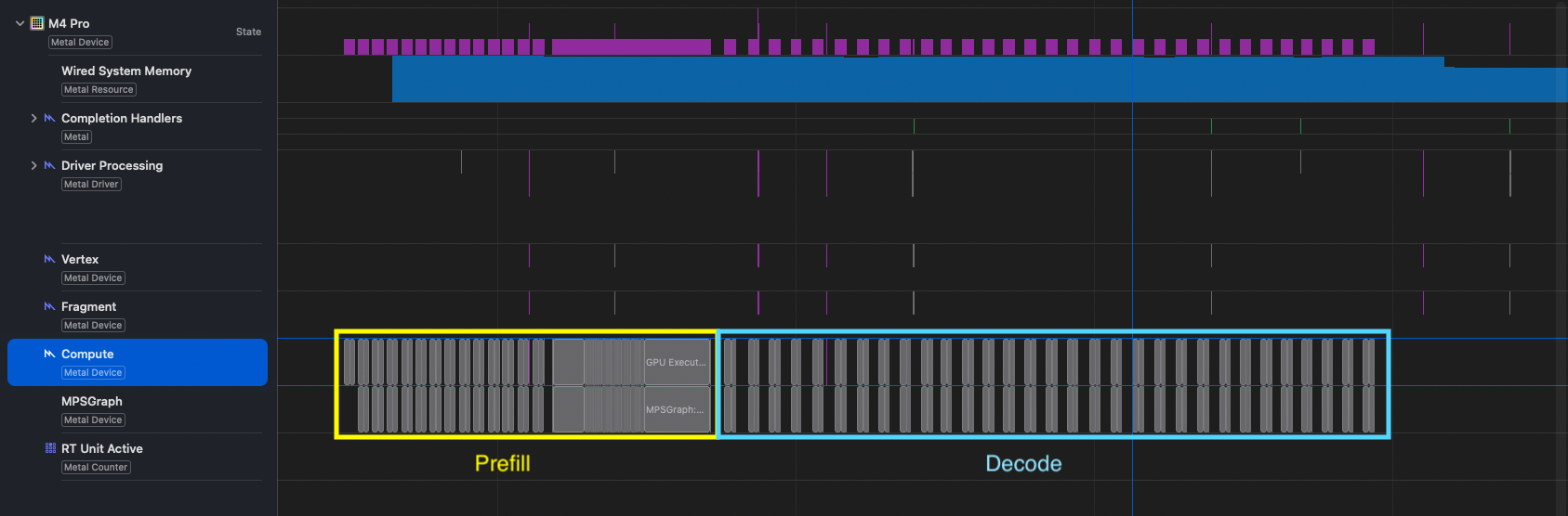
The prefill region is visually dense. The model applies large matrix operations across all prompt positions, exposing enough parallel work to keep the GPU busy.

Decode looks like a picket fence. Each iteration can begin only after the previous token has been selected, so batch-one generation repeatedly performs this sequence: CPU dispatch -> short GPU workload -> synchronize -> choose token -> repeat.

This shape is consistent with the usual roofline explanation: prefill has higher arithmetic intensity and is often compute-bound, whereas latency-sensitive, batch-one decode tends to be memory-bandwidth-bound. NVIDIA gives the same broad characterization in its LLM inference optimization guide.

There is an important limit to what this screenshot proves. A dense timeline is evidence that more GPU work was scheduled; it is not by itself an ALU-utilization percentage. Establishing the limiting resource requires GPU counters such as arithmetic/ALU activity, memory bandwidth, occupancy, and the reported limiter. The workload shape and counter evidence should agree before calling a phase compute- or memory-bound.

The PyTorch trace connected phases to resources

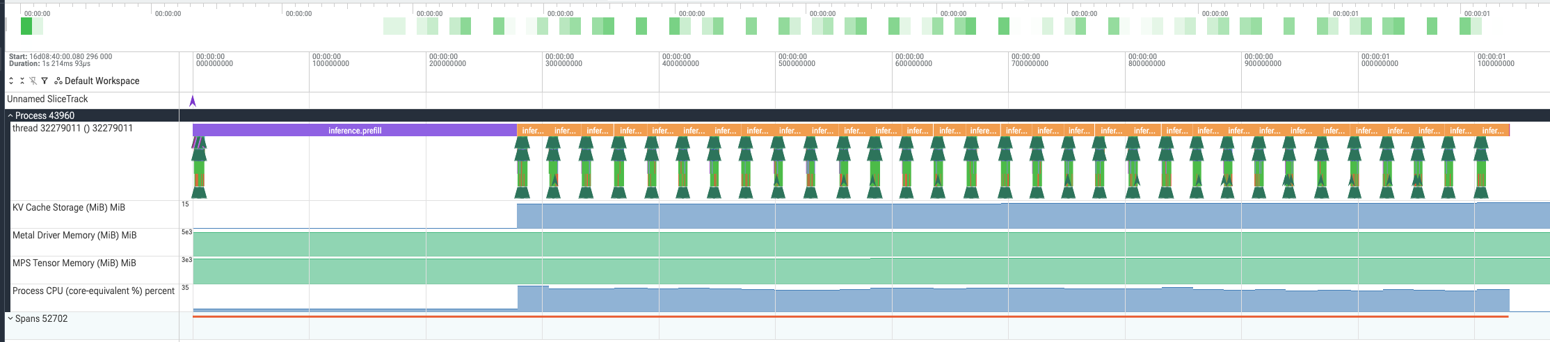
PyTorch’s mps backend maps operations to MPS Graph and tuned Metal Performance Shaders kernels. Unlike CUDA activity in PyTorch Profiler, MPS GPU execution is not represented as a native ProfilerActivity. I therefore used two complementary views:

• PyTorch record_function ranges for the logical prefill and decode stages.
• torch.mps.profiler.profile OS Signposts and a Metal capture for GPU-side inspection.

The profiling path in profile_generate() runs the same state machine rather than calling a different generation API. After prefill and after every decode step, it invokes this nested sampler from engine.py:

# Define a phase-boundary sampler inside profile_generate so it can share timer state.
def sample_resources(phase: str, step: int, cache: Any) -> None:
    # Allow this nested function to update the previous CPU and wall-clock timestamps.
    nonlocal previous_wall, previous_cpu
    # Read a wall-clock timestamp for calculating the completed phase's duration.
    current_wall = time.perf_counter()
    # Read process CPU time so waiting time is not counted as active CPU execution.
    current_cpu = time.process_time()
    # Calculate wall time since the previous phase-boundary sample.
    wall_delta = current_wall - previous_wall
    # Calculate CPU execution time consumed over the same interval.
    cpu_delta = current_cpu - previous_cpu
    # Select the allocator APIs that correspond to the active accelerator backend.
    if self.device.type == "mps":
        # Read bytes occupied by live tensors known to PyTorch's MPS allocator.
        allocated = torch.mps.current_allocated_memory()
        # Read total bytes currently allocated by the Metal driver for the process.
        driver_allocated = torch.mps.driver_allocated_memory()
    # Use the comparable allocated-versus-reserved CUDA counters on NVIDIA hardware.
    elif self.device.type == "cuda":
        # Read bytes occupied by live tensors on the selected CUDA device.
        allocated = torch.cuda.memory_allocated(self.device)
        # Read bytes held in PyTorch's CUDA caching allocator pool.
        driver_allocated = torch.cuda.memory_reserved(self.device)
    # Give CPU-only profiling an explicit zero rather than a misleading GPU value.
    else:
        # Record that no accelerator tensor allocation is available.
        allocated = 0
        # Record that no accelerator driver allocation is available.
        driver_allocated = 0
    # Append one structured sample aligned with the completed inference phase.
    resource_samples.append(
        ResourceSample(
            phase=phase,  # Identify before_prefill, after_prefill, or after_decode.
            step=step,  # Identify the decode iteration, with zero reserved for prefill.
            allocated_mib=allocated / (1024**2),  # Convert allocator bytes to MiB.
            driver_allocated_mib=driver_allocated / (1024**2),  # Convert pool bytes to MiB.
            cache_mib=_cache_size_bytes(cache) / (1024**2),  # Count unique KV tensor storage.
            process_cpu_percent=(  # Express CPU time as a core-equivalent percentage.
                cpu_delta / wall_delta * 100  # Divide active CPU seconds by wall seconds.
                if wall_delta and phase != "before_prefill"  # Avoid an invalid first interval.
                else 0.0  # Use zero before any inference phase has completed.
            ),
        )
    )
    # Carry this wall timestamp forward as the next interval's starting point.
    previous_wall = current_wall
    # Carry this CPU timestamp forward as the next interval's starting point.
    previous_cpu = current_cpu

I sampled three different memory concepts. Keeping them separate turned out to be essential.

Counter	What it means	What happened
KV cache storage	Bytes in the cache tensors reachable from past_key_values	0 -> 14.0 -> 14.8477 MiB
MPS tensor memory	Live tensor allocations known to PyTorch’s MPS allocator	2944.4 -> 2958.4 -> 2966.1 MiB
Metal driver memory	Total memory allocated by the Metal driver for this process	4534.7 -> 4588.7 MiB, then flat

The flat driver-memory line does not contradict the growing cache. Allocators reserve memory in larger blocks and reuse that pool for later tensor allocations. A logical tensor can grow while the driver’s already-reserved pool remains unchanged.

Likewise, 0 B in a PyTorch operator table’s CPU-memory column would not mean that Metal used no memory. It only means that particular CPU allocator counter did not observe the GPU allocation.

The strongest result: KV growth matched the architecture exactly

The raw samples were:

Phase	Step	KV cache (MiB)
before_prefill	0	0.000000
after_prefill	0	14.000000
after_decode	1	14.027344
after_decode	2	14.054688
…	…	…
after_decode	30	14.820312
after_decode	31	14.847656

Every decode step added 0.02734375 MiB, exactly 28 KiB per token. From the model configuration, KV bytes per token = layers × (key + value) × KV heads × head dimension × bytes per element = 28 × 2 × 2 × 128 × 2 = 28,672 bytes = 28 KiB.

For the 512-token prompt, 512 × 28 KiB = 14 MiB.

That is precisely the post-prefill measurement. After 31 additional decode passes, (512 + 31) × 28 KiB = 14.84765625 MiB.

Again, this is precisely the observed value.

This calculation also explains why grouped-query attention matters. Qwen2.5-1.5B has 12 query heads but only 2 KV heads. Cache size depends on the KV-head count, so storing keys and values for 2 heads is much cheaper than storing them for all 12 query heads.

---

What the CPU measurement does—and does not—say

The process used more CPU during the repeated decode loop than during the long prefill kernel. My phase samples were approximately 66% of one core for prefill and around 100% for most decode steps. Here, 100% means one core-equivalent, not the whole 14-core CPU.

My first explanation was that the CPU must be moving tensors from unified memory into the GPU cache. That is too literal and is not supported by the measurement.

On Apple silicon, the CPU and GPU can access the same physical allocation through unified memory. Apple describes Metal shared resources as CPU- and GPU-accessible without the traditional duplication between system RAM and video RAM. The processors still have private caches, and access still consumes memory bandwidth, but application code does not need the CPU to copy every model tensor into a separate VRAM allocation.

A safer interpretation is that decode creates more host orchestration per unit of GPU work:

• Python executes the autoregressive loop.
• PyTorch and MPS prepare and submit many small operations.
• Each step updates framework-side state and selects a token.
• This experiment deliberately synchronizes at every step.

Apple’s CPU/GPU synchronization guidance also makes the distinction clear: shared physical memory does not remove dependencies or stalls between processors.

CUDA versus Apple silicon during inference

First, this comparison needs precise language. CUDA is NVIDIA’s programming platform and software stack; Apple silicon is a family of systems-on-a-chip. The useful comparison for this experiment is therefore:

PyTorch CUDA backend + NVIDIA GPU versus PyTorch MPS backend + Metal + Apple GPU.

Architectural concern	CUDA on a typical discrete NVIDIA GPU	MPS/Metal on Apple silicon
Physical topology	CPU and GPU are commonly separate devices connected by PCIe or NVLink	CPU, GPU, Neural Engine, memory controllers, and other blocks share one SoC
Main memory	System RAM and GPU VRAM are normally distinct physical pools	One unified physical memory pool is available to CPU and GPU
Programming path	PyTorch -> ATen/CUDA libraries -> CUDA runtime/driver -> kernels	PyTorch -> MPS Graph/MPS kernels -> Metal driver -> GPU commands
Parallel hardware	Thread blocks run on Streaming Multiprocessors; Tensor Cores accelerate supported matrix operations	Threads execute in SIMD groups on Apple GPU cores; MPS supplies GPU-family-tuned kernels
CPU/GPU transfers	Explicit copies or managed/unified-memory migration may be required between host and device memory	Shared resources avoid the traditional RAM-to-VRAM copy, but still require synchronization and efficient access
ML accelerator in this experiment	NVIDIA Tensor Cores may be used by compatible CUDA kernels	The Apple GPU is used; selecting device="mps" does not mean the separate Neural Engine runs the model
PyTorch profiling	CPU and CUDA activities, kernel timing, and CUDA memory are integrated into PyTorch Profiler	CPU-side PyTorch activity is visible there; Metal Signposts, Instruments, and Metal Debugger supply GPU detail

NVIDIA’s CUDA Programming Guide describes the host/device model, Streaming Multiprocessors, and the host/device memory spaces. It also documents important exceptions to the simple “CUDA means separate VRAM” picture: CUDA can run on integrated SoCs, and systems such as Grace Hopper provide coherent unified-memory capabilities. The table describes the common discrete-GPU setup, not every CUDA machine.

Apple’s Metal compute guidance for Apple silicon explains the other side: unified memory removes the traditional need to maintain system-memory and video-memory copies. Metal’s shared storage mode gives both processors access to the same resource.

What stays the same

The transformer algorithm does not change with the backend:

• Prefill still produces the first token and the initial KV cache.
• Decode still has a sequential token dependency.
• The KV cache still grows linearly with layers, KV heads, head dimension, precision, batch size, and sequence length.
• Batch-one decode still has low arithmetic intensity compared with large prefill matrix operations.

What changes

The memory topology and software path change the cost and visibility of the work:

• A discrete CUDA system may pay explicit or managed migration costs across a CPU/GPU interconnect. Apple silicon usually avoids that separate-copy boundary.
• Apple unified memory lets a GPU address a large fraction of system memory, which is attractive for local models that would not fit in a smaller discrete VRAM pool.
• Unified capacity is not the same as unlimited bandwidth. During decode, weights and cache data still travel from DRAM through the memory hierarchy into GPU caches and execution units.
• CUDA exposes richer GPU activity directly through PyTorch Profiler. On MPS, correlating framework operations with GPU counters requires more than one tool.

Finally, the Apple Neural Engine should not be inferred from the words “Apple silicon” or “machine learning.” This experiment moved the model to torch.device("mps"), so it exercised the Apple GPU. Core ML is a different deployment path that may schedule supported operations across CPU, GPU, and Neural Engine.

---

Summary and learning takeaways

• Autoregressive generation is a state machine, not one model call. Prefill processes the complete prompt and produces the first output token; the remaining tokens are generated through sequential cached decode calls.
• Prefill and decode stress the hardware differently. Prefill exposes substantial parallel computation, while batch-one decode repeatedly launches smaller workloads and reads the model weights and expanding context for each token.
• KV caching trades computation for memory. In this experiment, the cache grew by exactly 28 KiB per cached token, matching the value derived from the model’s layers, KV heads, head dimension, and FP16 precision.
• On Apple silicon, this PyTorch MPS workload uses the CPU for orchestration and the Apple GPU for model computation. Unified memory removes the traditional RAM-to-VRAM copy boundary, but it does not remove synchronization, cache traffic, or memory-bandwidth limits. The Neural Engine was not used.
• A trustworthy explanation needs multiple views: application ranges identify the phase, synchronized timers measure latency, PyTorch shows framework operations, Metal counters describe GPU behaviour, and explicit tensor accounting reveals logical KV-cache growth. A profiler trace is diagnostic evidence rather than a clean benchmark result.