Deploying state-of-the-art neural networks to embedded or mobile edge devices is a constant battle against physical constraints. A standard VGG network trained on the CIFAR-10 dataset has a baseline accuracy of 92.95%, but it requires 35.20 MiB of storage and roughly 606 million Multiply-Accumulate (MAC) operations per image. On a resource-constrained microcontroller or mobile processor, this footprint is prohibitive.

To make these models viable on the edge, we turn to neural network pruning—the process of systematically removing parameters from the network while striving to preserve accuracy.

This post is a deep dive into two distinct pruning paradigms: Fine-Grained (Unstructured) Pruning and Channel (Structured) Pruning. We will walk through their PyTorch implementations, explore layer sensitivity profiles, and discuss the hardware trade-offs that dictate which method is best for real-world deployment.

---

Why Can We Prune? Weight Distribution Analysis

Before writing any pruning code, we need to understand why neural networks can lose a huge portion of their parameters and still function. The answer lies in the distribution of weight values.

If we look at the weight histograms of a trained VGG model, we find that the weights in almost all layers exhibit a zero-centered, bell-shaped (Gaussian-like) distribution.

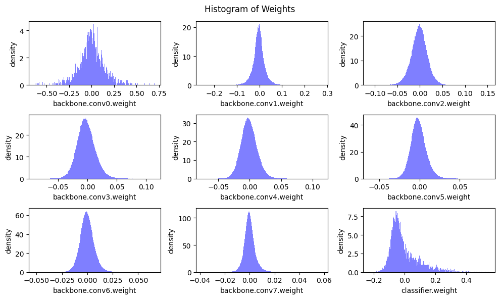
How this distribution helps pruning:

Because the majority of weights cluster tightly around zero, their absolute magnitudes are very small. In a neural network, a weight of 0.01 contributes almost nothing to the activation of the next layer compared to a weight of 0.8. Setting these near-zero weights to exactly zero—introducing sparsity—allows us to eliminate them without significantly changing the model’s output or dropping its accuracy.

---

Part 1: Fine-Grained (Unstructured) Pruning

Fine-grained pruning operates on individual weights. We set a target sparsity (e.g., 60%), find the threshold magnitude below which weights should be discarded, and create a binary mask.

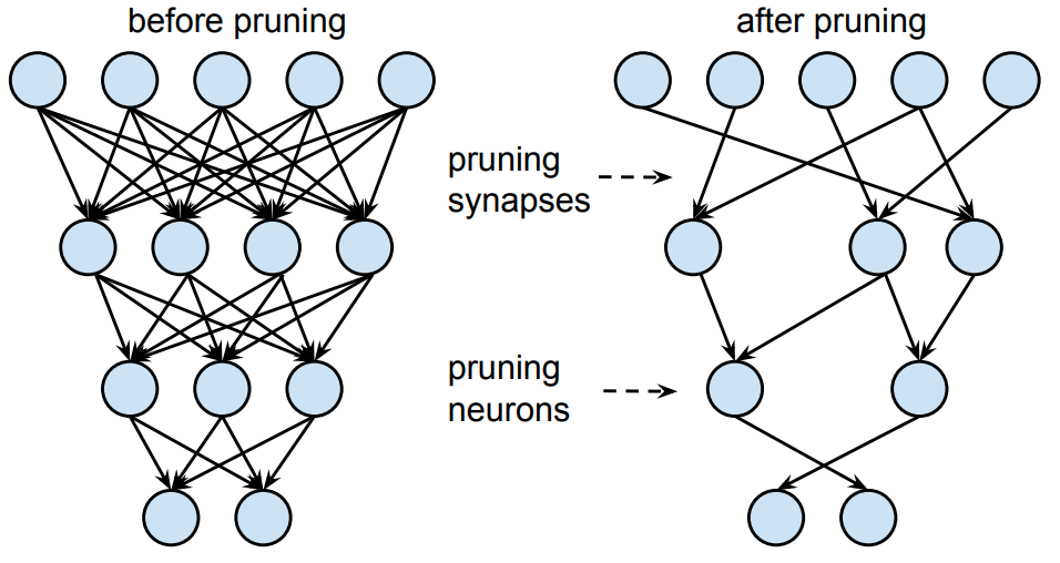
1. The PyTorch Implementation

Here is the magnitude-based fine-grained pruning implementation:

def fine_grained_prune(tensor: torch.Tensor, sparsity: float) -> torch.Tensor:
    """
    Prune a tensor in-place using magnitude-based fine-grained pruning.
    :param tensor: PyTorch tensor to be pruned.
    :param sparsity: Target sparsity ratio (between 0.0 and 1.0).
    :return: Binary mask indicating non-zero elements.
    """
    sparsity = min(max(0.0, sparsity), 1.0)
    if sparsity == 1.0:
        tensor.zero_()
        return torch.zeros_like(tensor)
    elif sparsity == 0.0:
        return torch.ones_like(tensor)

    num_elements = tensor.numel()

    # Step 1: Calculate the number of zeros to introduce
    num_zeros = round(sparsity * num_elements)
    
    # Step 2: Calculate the importance of weight (absolute magnitude)
    importance = torch.abs(tensor)
    
    # Step 3: Find the pruning threshold using the kth value
    threshold = importance.flatten().kthvalue(num_zeros)[0]
    
    # Step 4: Get binary mask (1 for nonzeros, 0 for zeros)
    mask = (importance > threshold).float()
    
    # Step 5: Apply mask to prune the tensor in-place
    tensor.mul_(mask)

    return mask

By applying this function, weights below the threshold magnitude are zeroed out, resulting in a sparse tensor.

2. Layer Sensitivity Analysis

Not all layers in a neural network are created equal. If we prune every layer to the same sparsity, accuracy drops quickly. To prune effectively, we must generate sensitivity curves by pruning one layer at a time to varying sparsities and recording the resulting accuracy.

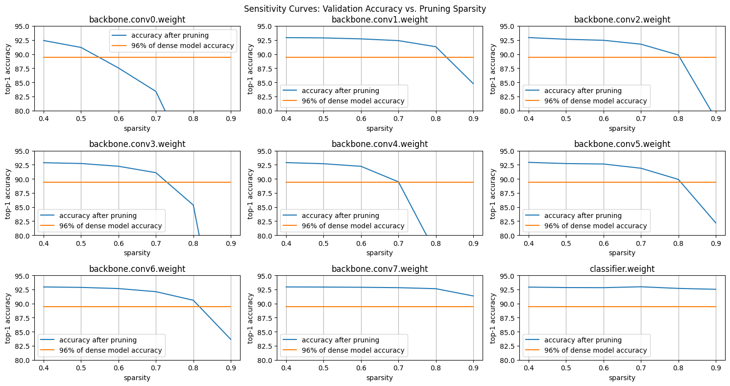
Layer Type	Sensitivity Level	Why?
First Layer (conv0)	Extremely High	It processes raw pixels and extracts low-level features (edges, textures). Since it has only 3 input channels, there is zero redundancy; pruning it destroys basic vision details.
Intermediate Convs	Moderate	Mid-level layers have more channels and exhibit moderate redundancy, letting us prune them up to 40-50% before accuracy begins to degrade.
Final Classifier	Low (Very Robust)	The final linear layer contains the bulk of the network parameters (redundancy is very high) and maps abstract concepts. We can prune it to 90% sparsity with virtually no accuracy loss.

3. Layer-by-Layer Sparsity Allocation

Based on sensitivity curves and parameter distributions, we formulate a non-uniform layer-by-layer sparsity plan to maximize compression:

sparsity_dict = {
    'backbone.conv0.weight': 0.4,  # Sensitive first layer: prune conservatively
    'backbone.conv1.weight': 0.7,  # Larger, less sensitive
    'backbone.conv2.weight': 0.5,
    'backbone.conv3.weight': 0.4,
    'backbone.conv4.weight': 0.4,
    'backbone.conv5.weight': 0.4,
    'backbone.conv6.weight': 0.4,
    'backbone.conv7.weight': 0.8,  # High redundancy in deep layer
    'classifier.weight': 0.9       # Classifier has the most parameters: prune aggressively
}

Applying this plan and counting only non-zero weights, the model shrinks from 35.20 MiB to 17.32 MiB — 49.2% of the dense size (roughly a 2× reduction). The accuracy story shows why fine-tuning matters:

• Right after pruning (before fine-tuning): 90.84% — a noticeable drop from the dense 92.95%.
• After 5 epochs of fine-tuning: 92.82% — a drop of only 0.13% from the dense baseline.

The mask is re-applied after every optimizer step so the network stays sparse throughout fine-tuning, letting the surviving weights compensate for the ones we removed.

---

Part 2: Channel (Structured) Pruning

While fine-grained pruning is elegant, it has a fatal flaw: standard CPUs and GPUs cannot easily accelerate sparse matrix multiplication. To achieve real speedups without custom hardware, we use Channel Pruning to physically shrink the dimensions of the tensors.

Fine-Grained Pruning (Unstructured):
[ W  0  W  0 ]  <- Keeps shape, introduces zeroes.
[ 0  W  0  W ]     Requires sparse computing support.

Channel Pruning (Structured):
[ W  W  W ]     <- Physically deletes channels (filters).
[ W  W  W ]        Produces a smaller, dense matrix.

1. Dimension Alignment in PyTorch

When we prune an output channel of a convolutional layer, we must also prune:

1. The corresponding scale, bias, and running statistics of its associated BatchNorm layer.
2. The matching input channels of the succeeding convolutional layer.

Here is the structured channel pruning implementation:

def get_num_channels_to_keep(channels: int, prune_ratio: float) -> int:
    return int(round(channels * (1. - prune_ratio)))

@torch.no_grad()
def channel_prune(model: nn.Module, prune_ratio: Union[List, float]) -> nn.Module:
    # prune_ratio can be a single float (uniform across layers) or a per-layer list.
    n_conv = len([m for m in model.backbone if isinstance(m, nn.Conv2d)])
    if isinstance(prune_ratio, list):
        assert len(prune_ratio) == n_conv - 1
    else:  # convert a uniform float into a per-layer list
        prune_ratio = [prune_ratio] * (n_conv - 1)

    model = copy.deepcopy(model)
    all_convs = [m for m in model.backbone if isinstance(m, nn.Conv2d)]
    all_bns = [m for m in model.backbone if isinstance(m, nn.BatchNorm2d)]
    
    for i_ratio, p_ratio in enumerate(prune_ratio):
        prev_conv = all_convs[i_ratio]
        prev_bn = all_bns[i_ratio]
        next_conv = all_convs[i_ratio + 1]
        
        original_channels = prev_conv.out_channels
        n_keep = get_num_channels_to_keep(original_channels, p_ratio)

        # Prune the output of the previous conv and bn
        prev_conv.weight.set_(prev_conv.weight.detach()[:n_keep])
        prev_bn.weight.set_(prev_bn.weight.detach()[:n_keep])
        prev_bn.bias.set_(prev_bn.bias.detach()[:n_keep])
        prev_bn.running_mean.set_(prev_bn.running_mean.detach()[:n_keep])
        prev_bn.running_var.set_(prev_bn.running_var.detach()[:n_keep])

        # Prune the input of the next conv to align dimensions
        next_conv.weight.set_(next_conv.weight.detach()[:, :n_keep])

    return model

2. Structured Selection: Channel Sorting by Importance

Naively keeping the first K channels is suboptimal. We want to keep the channels that contain the most information. We compute the importance of each input channel based on the L₂ norm of its weights, $\lVert \mathbf{w}_c \rVert_2 = \sqrt{\sum_i w_{c,i}^{\,2}}$, sort the channels, and keep the top ones:

def get_input_channel_importance(weight: torch.Tensor) -> torch.Tensor:
    importances = []
    # Compute the L2 norm for each input channel
    for i_c in range(weight.shape[1]):
        channel_weight = weight.detach()[:, i_c]
        importance = torch.norm(channel_weight)  # L2 norm
        importances.append(importance.view(1))
    return torch.cat(importances)

@torch.no_grad()
def apply_channel_sorting(model: nn.Module) -> nn.Module:
    model = copy.deepcopy(model)
    all_convs = [m for m in model.backbone if isinstance(m, nn.Conv2d)]
    all_bns = [m for m in model.backbone if isinstance(m, nn.BatchNorm2d)]
    
    for i_conv in range(len(all_convs) - 1):
        prev_conv = all_convs[i_conv]
        prev_bn = all_bns[i_conv]
        next_conv = all_convs[i_conv + 1]
        
        # Sort channels based on input channel importance in the next layer
        importance = get_input_channel_importance(next_conv.weight)
        sort_idx = torch.argsort(importance, descending=True)

        # Apply sorted index to previous conv and bn
        prev_conv.weight.copy_(torch.index_select(prev_conv.weight.detach(), 0, sort_idx))
        for tensor_name in ['weight', 'bias', 'running_mean', 'running_var']:
            tensor_to_apply = getattr(prev_bn, tensor_name)
            tensor_to_apply.copy_(torch.index_select(tensor_to_apply.detach(), 0, sort_idx))

        # Apply sorted index to next conv input weights
        next_conv.weight.copy_(torch.index_select(next_conv.weight.detach(), 1, sort_idx))

    return model

Sorting ensures that the channels with the largest weight magnitudes are grouped at the beginning, allowing us to drop the less important ones from the end. Importantly, channel sorting is an equivalence-preserving transform — reordering channels (and the matching weights of the next layer) does not change the network’s output, so the dense model’s accuracy stays at 92.95% before and after sorting.

3. The Accuracy Cliff — and Why Fine-Tuning Is Mandatory

Channel pruning is far more destructive than fine-grained pruning, because deleting a whole filter removes every weight it contains, important or not. Pruning just 30% of channels illustrates the cliff:

Stage	Accuracy
Dense baseline	92.95%
Pruned 30%, no sorting	28.14%
Pruned 30%, with channel sorting	36.81%
Pruned 30% + sorting, after 5 epochs of fine-tuning	92.30%

Two lessons fall out of this:

1. Sorting helps, but only a little on its own. Keeping the high-L₂-norm channels lifts accuracy from 28.14% to 36.81% — better, but still a collapsed model.
2. Fine-tuning does the heavy lifting. Recovery from ~37% back to 92.30% comes almost entirely from re-training the smaller, dense network. Unlike fine-grained pruning (0.13% drop), channel pruning leaves a 0.65% residual gap even after fine-tuning — the price of a physically smaller tensor.

4. Performance Analysis: MACs vs. Latency Speedup

Applying a 30% uniform channel pruning ratio and running the model on CPU (simulating an edge device), the actual measured results from the lab are:

                Original        Pruned          Reduction Ratio
Latency (ms)    17.3            10.2            1.7
MACs (M)        606             305             2.0
Param (M)       9.23            5.01            1.8

First, notice that a 30% channel pruning ratio produces a ~2× (50%) MAC reduction, not 30%. This is because pruning compounds across consecutive layers: the MACs of a convolution are proportional to $C_{\text{in}} \times C_{\text{out}}$, and channel pruning shrinks both — the pruned output channels of one layer become the pruned input channels of the next. Keeping 70% of channels on each side gives roughly $0.7 \times 0.7 \approx 0.49$ of the original computation, i.e. about half.

But while MACs are cut in half (2×) and parameters drop by nearly half too, the wall-clock latency only improves by 1.7×, not 2×. Why?

The key insight is that channel pruning only shrinks the convolution work — not everything else in the network. This is essentially Amdahl’s law: the operations that don’t shrink come to dominate the runtime.

1. Un-pruned operations: BatchNorm, pooling, activation functions, and the final linear classifier are not “pruned” the way convolutions are. Their inputs may be slightly smaller, but their fundamental cost — memory access, control flow, fixed per-op overhead — does not scale down proportionally with channel count.
2. A larger residual fraction: As convolutional MACs collapse, these fixed-cost operations become a larger share of the total inference time. So even though the heavy conv math is halved, end-to-end latency can’t fall as fast as the raw MAC count.

Note on hardware: These measurements were taken on CPU (simulating an edge device). On a GPU you would see additional factors — warp occupancy, kernel-launch overhead, and memory bandwidth — but those are specific to GPU execution and do not apply to this CPU benchmark.

---

Part 3: The Grand Trade-Off: Unstructured vs. Structured

When designing an EfficientML pipeline, choosing between fine-grained (unstructured) and channel (structured) pruning comes down to the following trade-offs:

Metric	Fine-Grained Pruning	Channel Pruning
Accuracy at High Sparsity	High (Robust)	Low (Sensitive)
Hardware Acceleration	Requires Sparse Hardware	Native (CPUs, GPUs, TPUs)
Real Latency Speedup	Zero on standard libraries	Immediate, near-linear
Memory Storage Overhead	Requires metadata (CSR indices/masks)	Zero (Native dense shape)

Key Takeaway

• Use Fine-Grained Pruning if you are targeting specialized edge AI accelerators (like NVIDIA Tensor Cores with 2:4 sparsity support) and cannot tolerate any accuracy loss.
• Use Channel Pruning if you need immediate, out-of-the-box latency speedup on standard CPUs, GPUs, or browser-based ONNX runtimes, and have enough training budget to recover lost accuracy through fine-tuning.