Deploying a state-of-the-art neural network to a phone or microcontroller means fighting for every megabyte and every millijoule. Our baseline VGG network, trained on CIFAR-10, reaches 92.95% accuracy — but it stores all 9.2 million weights as 32-bit floats, for a footprint of 35.20 MiB. On the edge, that’s often too big to ship.

Quantization attacks this directly: instead of storing each weight in 32 bits, we represent it with far fewer — 8 bits, 4 bits, sometimes 2 — shrinking the model 4×, 8×, or more, and (on the right hardware) speeding up inference by replacing floating-point math with integer math.

This post is a lab-driven deep dive into two quantization families — K-Means (codebook) Quantization and Linear (affine) Quantization — and the cross-cutting choice that governs how much accuracy you keep: post-training quantization (PTQ) vs. quantization-aware training (QAT).

---

Why can we get away with it?

The same reason pruning works: trained weights carry far less information than 32 bits implies.

FP32 is a galaxy-sized ruler

An FP32 number spends its bits on a huge dynamic range — it can represent magnitudes from about 10⁻³⁸ to 10³⁸ — plus roughly 7 digits of precision. But if you drop all 9.2M trained weights onto a number line, they don’t spread out. They pile into a narrow, zero-centered bell, almost all within −0.5…0.5.

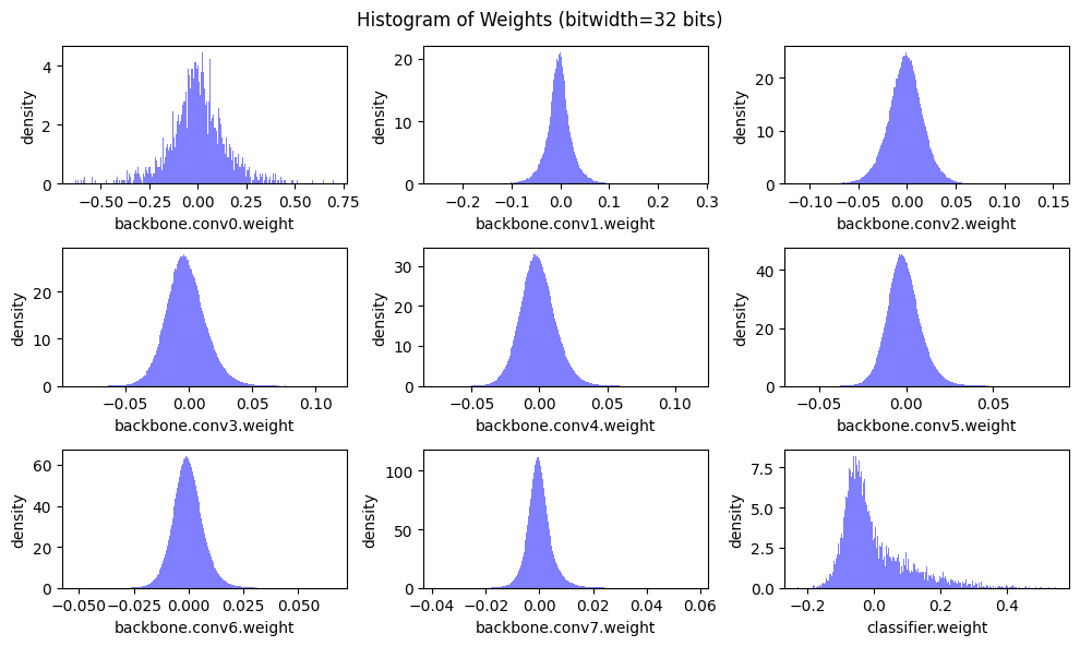
It’s like owning a ruler that measures from the width of an atom to the distance to the Moon, then only ever using it to measure coins. The instrument works — but nearly all of its range is wasted. FP32 is that ruler; the weights are the coins.

So we stop describing weights in absolute, galaxy-scale units. We pick the smallest step we care about — one shared scale for the tensor — and just record how many steps from zero each weight is. Each weight becomes a small integer, and the wasted range is gone.

Why losing precision barely hurts

With 8 bits we keep 256 distinct levels across the weight band, so each weight is snapped to its nearest level — off by at most half a tiny step. Two things then make that error nearly free:

1. The decision is an argmax over 10 classes. When the network is confident, small wiggles in the output don’t change which class is largest.
2. The errors cancel. A neuron sums hundreds of weight × input terms. The rounding errors are random and roughly zero-mean, so across the sum they largely cancel — the signal grows like $N$, but the noise only like $\sqrt{N}$.

The one idea to remember: quantization adds a small, zero-mean noise to each weight, and a wide network averages that noise away — right up until the noise gets too big to average away.

That threshold is exactly what the numbers show:

Bit-width	Distinct levels	Accuracy
32 (FP32 baseline)	—	92.95%
8-bit	256	92.76%
4-bit	16	79.07%
2-bit	4	10.00%

256 levels keeps the per-weight error small enough to average away. Sixteen levels starts to pinch. Four levels blows past the threshold — the dot products turn to noise and the model degrades to random guessing. Everything else in this post is about pushing the bit-width down while clawing that accuracy back.

(These are k-means quantization results, measured in the lab; the same intuition carries over to linear quantization in Part 2.)

---

PTQ vs. QAT: the choice that runs through everything

Every quantization method has to answer one question: do we let training see the quantization, or not? That single fork defines the two regimes you’ll see throughout this post.

Post-training quantization (PTQ) takes an already-trained model and quantizes it once, afterward. It may run a handful of batches through the network to calibrate — measuring activation ranges so it can choose a good scale and zero_point — but that’s measurement, not learning. The model never experienced quantization during training. It’s cheap (seconds to minutes), needs no labels, and is the first thing you should try.

Quantization-aware training (QAT) simulates quantization inside the training forward pass. A “fake-quantize” node rounds the weights (and activations) on every forward step, so the loss is computed on quantized values and the gradients push the weights toward positions where that error does the least damage. It costs a real training run, but it recovers accuracy that PTQ leaves on the floor.

The dividing line is not “did backprop happen?” — it’s was quantization present in the forward pass while you trained? Fine-tune a full-precision model and quantize it afterward, and that’s still PTQ no matter how much backprop you did. Fine-tune with the weights kept quantized every forward step, and that’s QAT. Same optimizer, same gradients — what flips the label is whether the rounding was in the loop.

PTQ comes in three flavors

That single “quantize once” box above isn’t one thing. Once you’ve decided not to retrain, you still have to answer a second question: what do you quantize ahead of time, and where do the activation ranges come from? That fork expands the PTQ box into three flavors — and the two labs in this post are each a different one.

Flavor	Weights	Activations	Calibration data?	Compute runs in
Dynamic	quantized offline	quantized at runtime, per-inference	No	int matmul + live range-calc each call
Static	quantized offline	quantized offline (fixed S, Z)	Yes	full integer, end-to-end
Weight-only	quantized offline	left in FP16 / FP32	No	float (weights dequantized first)

Dynamic freezes the weights to int8 offline but quantizes each activation tensor on the fly — every inference measures the real min/max and picks a fresh scale/zero_point, so it never has to guess a range and needs no calibration set. The cost is per-call overhead. It’s the default for LSTMs and Transformers, where activation ranges swing hard between inputs.

Static bakes fixed scale/zero_point into both weights and activations. Since you commit to activation ranges offline, you need a calibration pass: run a few hundred representative batches, observe the activation histograms, and pick ranges (min/max, percentile, or KL-divergence). After that everything is integer at runtime — no per-call range math, and the only flavor that’s truly integer-only end-to-end. This is the linear int8 path in this post — the “handful of batches to calibrate” above is exactly the static-PTQ calibration step.

Weight-only quantizes just the weights (often int4/int3) and leaves activations in FP16; at compute time the weights are dequantized back to float and the matmul runs in float. There’s no integer-compute speedup — the win is pure memory and bandwidth, because you load 4-bit weights instead of 32-bit. It dominates LLM serving (GPTQ, AWQ), where the bottleneck is fetching a giant weight matrix, not the arithmetic. The k-means codebook lab is morally weight-only: it compresses storage, and weights are decompressed for compute — which is why the codebook scheme unlocks storage compression while linear unlocks integer compute.

The “graph update” that static needs (and the others mostly don’t). Static PTQ isn’t just picking numbers — it rewrites the model graph: insert quant/dequant nodes (QuantStub/DeQuantStub) at the integer-domain boundaries, fuse Conv → BN → ReLU into a single int kernel so you don’t round-trip to float between layers, and swap each op for its integer kernel. In PyTorch that’s the prepare() (insert observers, calibrate) → convert() (rewrite to int kernels) two-step. Dynamic skips calibration and the heavy fusion; weight-only just repacks the weight tensors and leaves the activation graph in float.

So the one-line mental model: dynamic = quantize weights, measure activations live; static = quantize everything offline + calibrate + fuse the graph (← the int8 lab); weight-only = quantize weights only, for memory (← the codebook lab).

How do you choose? Set an accuracy budget.

Try PTQ first; escalate to QAT only if the accuracy drop exceeds what you can tolerate. The lab makes this literal with a 0.5% drop threshold:

Bit-width	Accuracy after PTQ	Drop	Verdict
8-bit	92.76%	0.19%	Under budget → PTQ is enough
4-bit	79.07%	13.88%	Over budget → QAT → 92.55%
2-bit	10.00%	82.95%	Over budget → QAT → 91.25%

The trick that makes QAT possible: the Straight-Through Estimator

There’s a problem hiding in QAT: rounding is a step function, so its gradient is zero almost everywhere (and undefined at the steps). Backprop through it would zero out every gradient, and the model could never learn. The fix is the Straight-Through Estimator (STE):

Round in the forward pass so the network feels the quantization error — but on the backward pass, pretend the rounding was the identity function and let the gradient pass straight through it. Those gradients update a full-precision “shadow” copy of the weights, which is re-quantized on the next step.

So QAT always keeps the real, continuous weights around: quantization happens on the forward pass, and learning happens in full precision. In the k-means variant we’ll see in Part 1, the same idea appears as centroids that are recomputed as the mean of the weights assigned to each cluster — the codebook chases the weights as they move.

What fake-quantize actually does to one value

A fake-quant node is the heart of QAT, and the operation itself is tiny: take a float, snap it to the nearest grid point, hand back a float. Nothing becomes int8 — input and output are both FP32; only the value changes. Plotted, the forward pass is a staircase:

The catch the diagram makes obvious: the staircase is flat almost everywhere, so its real derivative is 0 — plain backprop would zero out every gradient and the model could never learn. The STE’s whole job is to lie on the backward pass and pretend the step was that straight diagonal, so the gradient passes through unchanged.

That’s also why the weights must stay FP32 during training, which is the part that’s easy to miss:

• A gradient step is a tiny nudge, say w -= 0.0007. If the grid spacing S is 0.004, that nudge is smaller than one step. Had w been stored as int8, 0.0007 would round to zero and the weight could never move.
• So you keep a full-precision master copy of w. Those sub-step nudges accumulate in it across many batches until w finally crosses into the next bin — at which point the fake-quant output jumps to the next step. The float weight glides; the value it emits moves in discrete hops.

So during training you carry both: an FP32 master weight that gradients update, and the fake-quant view of it that the loss sees. That FP32 master weight is the “continuous thing for gradients to flow through” — it exists precisely so tiny updates aren’t lost to rounding.

Same network, two dtypes: what actually flows between layers

A trap worth calling out: during QAT, are the activations between layers already INT8? No. You have to keep two pictures separate — what flows while you train, and what flows once you deploy — because they differ in dtype even when the numbers look identical.

• During QAT training, every tensor — inputs, weights, activations — is still stored as FP32. As the staircase above showed, fake-quant only rounds each value onto the int8 grid (0.1234567 → 0.1250000): the numbers look as coarse as int8, but the dtype stays float and every op runs in full precision (so gradients have somewhere continuous to land).
• At deployment, the fake-quant nodes are swapped for real quantize ops. One Quantize op at the very front turns the FP32 input (e.g. a camera frame) into int8; from there each layer consumes int8 and emits int8, with no float in the hot path. Only that first input conversion (and, at the end, a dequant of the logits) ever touches float.

So “the activations are int8” is true of the deployed model, not the QAT training run. During training they’re FP32 carrying int8-grid values; the int8 only becomes physically real at the convert step below.

The two regimes, in code

Let’s make the fork concrete on linear int8 — the regime production toolchains (TFLite, TensorRT, ONNX Runtime) are built around, and the one you’ll reach for first in practice.

PTQ never trains. It runs a few batches to calibrate — observe the value ranges — picks a scale and zero_point, and quantizes once:

model = trained_fp32_model                           # 92.95%

# 1. Calibrate: observe weight/activation ranges over a few batches (measurement, not learning)
ranges = collect_ranges(model, calib_loader)

# 2. Pick S and Z from those ranges, then quantize the weights once
for layer in model.quantizable_layers():
    S, Z = choose_scale_zero_point(ranges[layer], bitwidth=8)
    layer.weight_int = linear_quantize(layer.weight, bitwidth=8, scale=S, zero_point=Z)

accuracy = evaluate(quantized_model, test_loader)    # 92.87% — no gradients, no training

QAT simulates that int8 rounding inside the forward pass, so the loss feels it and the gradients can compensate. A “fake-quantize” op rounds-then-dequantizes, and the STE makes its backward an identity:

# Illustrative: the lab implements QAT only for k-means. Linear QAT uses this same
# fake-quant + STE recipe — which production toolchains (torch.ao.quantization, etc.) automate.

def fake_quantize(w, S, Z, q_min, q_max):
    q     = torch.clamp(torch.round(w / S) + Z, q_min, q_max)
    w_hat = (q - Z) * S                       # quantize → dequantize: snapped to the int8 grid, still float
    return w + (w_hat - w).detach()           # STE: forward = w_hat, backward = identity

# ── THIS is "using QAT": a layer that fake-quantizes its weight inside forward() ──
class QATLinear(nn.Linear):                   # (a QATConv2d looks the same)
    def forward(self, x):
        w_fq = fake_quantize(self.weight, self.S, self.Z, self.q_min, self.q_max)  # ← rounding enters the forward
        return F.linear(x, w_fq, self.bias)   # the matmul runs on the fake-quantized weight

# QAT is fine-tuning, not training from scratch: start from the SAME trained FP32 checkpoint PTQ used.
model = trained_fp32_model                    # the 92.95% model from ordinary FP32 training
attach_fake_quant(model)                      # swap each nn.Linear / nn.Conv2d → its QAT* version above
optimizer = torch.optim.SGD(model.parameters(), lr=0.01, momentum=0.9)  # low LR — fine-tuning

for epoch in range(num_finetune_epochs):      # a handful of epochs, not dozens
    for inputs, targets in train_loader:
        optimizer.zero_grad()
        outputs = model(inputs)               # every QAT layer calls fake_quantize() here — loss sees the rounding
        loss = criterion(outputs, targets)
        loss.backward()                       # STE routes the gradient to the FP32 weights
        optimizer.step()                      # update the full-precision shadow weights

# ── Convert: NOW the model actually becomes integer (this is the only step that shrinks it) ──
for layer in model.quantizable_layers():
    layer.weight_int = linear_quantize(layer.weight, bitwidth=8,   # real int storage, not float w_hat
                                       scale=layer.S, zero_point=layer.Z)
    del layer.weight                          # drop the FP32 weight; keep weight_int + S + Z

Note the bit-width lives in the fake_quantize range during training and in this linear_quantize call at convert — set both to 4 and you get an int4 model instead. Everything up to the convert line keeps the weights in FP32; fake_quantize only simulates the rounding (quantize → dequantize back to float). The model physically shrinks to integers only at that last loop.

The “use” of QAT is QATLinear.forward calling fake_quantize() on its weight before the matmul — that single line is what puts rounding inside the forward pass. attach_fake_quant just swaps every nn.Linear / nn.Conv2d for its QAT* version, so when model(inputs) runs, every layer rounds its weights on the fly. The original FP32 weights are never overwritten (self.weight stays full-precision); only the value used in the matmul is rounded, while optimizer.step() keeps refining self.weight underneath. After fine-tuning you run the real, non-fake quantization once and deploy.

The one line that makes it work is w + (w_hat - w).detach(). The forward value is the rounded w_hat, but .detach() hides the rounding from autograd, so ∂(output)/∂w = 1 and the gradient passes straight through to the full-precision w — the STE, in a single expression. PTQ is the same picture with the training loop deleted: calibrate, quantize once, deploy.

---

Part 1: K-Means Quantization

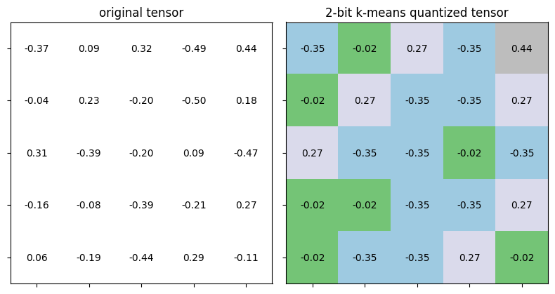
K-means quantization asks: across this whole tensor, what are the 2ⁿ values that best summarize all the weights? It runs k-means clustering on the weights, finds those 2ⁿ cluster centers (centroids), and replaces every weight with the centroid of its cluster.

The result is stored as a codebook — a lookup table, not a formula:

weights:    [ 0.21, -0.34,  0.19, -0.31,  0.02, ... ]
                 │  k-means clustering into 2ⁿ groups
                 ▼
labels:     [   2,    0,     2,    0,     1,   ... ]   ← n-bit index, stored per weight
centroids:  { 0: -0.32,  1: 0.01,  2: 0.20,  3: ... } ← the codebook, stored once
                 │  decode:  quantized = centroids[labels]
                 ▼
quantized:  [ 0.20, -0.32,  0.20, -0.32,  0.01, ... ]

The centroid is the quantized value; the label is just an index into the table — there is no scale factor or arithmetic, only a lookup.

The implementation

from collections import namedtuple
Codebook = namedtuple('Codebook', ['centroids', 'labels'])

def k_means_quantize(fp32_tensor, bitwidth=4, codebook=None):
    if codebook is None:
        # n-bit quantization → 2^n clusters
        n_clusters = 2 ** bitwidth
        kmeans = KMeans(n_clusters=n_clusters, mode='euclidean')
        labels = kmeans.fit_predict(fp32_tensor.view(-1, 1))
        centroids = kmeans.centroids.view(-1)
        codebook = Codebook(centroids, labels)
    # decode: replace each weight with its cluster's centroid
    quantized_tensor = codebook.centroids[codebook.labels]
    fp32_tensor.set_(quantized_tensor.view_as(fp32_tensor))
    return codebook

The number of clusters is 2 ** bitwidth — so 4-bit quantization produces exactly 16 distinct values (and 2ⁿ in general). Everything else is one line of decoding: index the centroid table with the labels.

What it costs to store

The saving is purely the per-weight index width. Each weight becomes an n-bit label instead of a 32-bit float; the codebook itself (2ⁿ floats) is negligible. So the compression ratio is just 32/n:

Bit-width	Size	Compression	Accuracy (PTQ)
FP32	35.20 MiB	1×	92.95%
8-bit	8.80 MiB	4×	92.76%
4-bit	4.40 MiB	8×	79.07%
2-bit	2.20 MiB	16×	10.00%

Recovering accuracy: k-means QAT

8-bit is fine straight out of PTQ (−0.19%). But 4-bit and 2-bit need quantization-aware training. The k-means flavor of QAT alternates two steps each epoch:

1. Forward on quantized weights — the network runs on the centroid values, so the loss feels the quantization error; STE passes gradients through to the full-precision weights.
2. Update the codebook — recompute each centroid as the mean of the (now-updated) weights assigned to it:

def update_codebook(fp32_tensor, codebook):
    n_clusters = codebook.centroids.numel()
    for k in range(n_clusters):
        codebook.centroids[k] = fp32_tensor[codebook.labels == k].mean()

The mean is not arbitrary: for a fixed cluster assignment, the mean is the value that minimizes the squared quantization error Σ(wᵢ − c)². So each update provably tightens the codebook around the weights. The recovery is dramatic:

• 4-bit: 79.07% → 92.55% (one epoch was enough to get under the 0.5% budget).
• 2-bit: 10.00% → 91.25% after 5 epochs — from random guessing back to a usable model, with only 4 distinct weight values.

---

Part 2: Linear Quantization

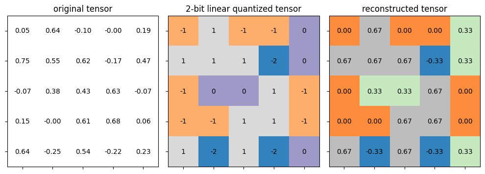
K-means compresses storage but still computes in floating point. Linear quantization is built to do the opposite: run the actual arithmetic in integers. It maps real values to integers with a simple affine rule:

$$\hat{r} = S\,(q - Z) \quad\text{(dequantize)}, \qquad q = \operatorname{clamp}\!\big(\operatorname{round}(r / S) + Z,\; q_{\min},\, q_{\max}\big) \quad\text{(quantize)}$$

• S (scale) — a float: the real-world size of one integer step.
• Z (zero-point) — an integer: the code that represents real 0.0 exactly.

Z exists so zero is represented without error, and so an asymmetric range (like an all-positive ReLU output) can use the full integer span instead of wasting half of it on values that never occur. When the range is symmetric, Z = 0.

Choosing the parameters: computing S and Z

S and Z fall out of two ranges — the float range the tensor actually occupies and the integer range the bit-width gives you. Four steps:

1. Observe the float range $[\,r_{\min}, r_{\max}\,]$. For weights you read it straight off the tensor (you already have them). For activations you can’t know it until data flows, so you calibrate: push a few batches through and record the min/max (static PTQ), or measure it live per batch (dynamic).
2. Fix the integer range $[\,q_{\min}, q_{\max}\,]$ from the bit-width and signedness — signed int8 → $[-128, 127]$; unsigned uint8 (e.g. a ReLU output that’s never negative) → $[0, 255]$.
3. Scale — how much real value one integer step covers: $S = \dfrac{r_{\max} - r_{\min}}{q_{\max} - q_{\min}}$
4. Zero-point — the integer code that maps exactly onto real 0.0, clamped into range: $Z = \operatorname{clamp}\!\big(\operatorname{round}(q_{\min} - r_{\min}/S),\; q_{\min}, q_{\max}\big)$

scale = (fp_max - fp_min) / (quantized_max - quantized_min)
zero_point = round(quantized_min - fp_min / scale)
zero_point = max(quantized_min, min(quantized_max, zero_point))  # clamp

Worked example (an asymmetric activation, signed int8). Suppose a layer’s outputs land in [−2.0, 6.0] and the target is int8 [−128, 127]:

• $S = \dfrac{6.0 - (-2.0)}{127 - (-128)} = \dfrac{8.0}{255} \approx 0.0314$
• $Z = \operatorname{round}\!\big(-128 - (-2.0 / 0.0314)\big) = \operatorname{round}(-128 + 63.7) = \operatorname{round}(-64.3) = -64$

So real 0.0 is stored as the code −64, and each integer step is worth ≈ 0.0314. Symmetric shortcut: when the range is symmetric (the usual case for weights), set $Z = 0$ and $S = \max(|r|) / q_{\max}$. No offset is needed — and a zero Z also drops terms from the integer matmul below, making inference cheaper.

With S and Z in hand, quantizing is the affine rule, rounded and clamped:

def linear_quantize(fp_tensor, bitwidth, scale, zero_point, dtype=torch.int8):
    # q = round(r / S) + Z, clamped to the integer range
    scaled  = fp_tensor / scale
    rounded = torch.round(scaled)
    shifted = rounded + zero_point
    q_min, q_max = get_quantized_range(bitwidth)
    return shifted.clamp(q_min, q_max).to(dtype)

Integer-only inference: the factoring trick

The payoff is that a whole layer can run in integer arithmetic. A linear/conv layer accumulates Σ rᵥᵥ·rₓ; substitute the affine form and the scales fall out of the sum:

Σ rᵥᵥ·rₓ = Sᵥᵥ·Sₓ · Σ (qᵥᵥ − Zᵥᵥ)(qₓ − Zₓ)
                      └── integer multiply-accumulate ──┘

The inner dot product is pure integers; the float scale Sᵥᵥ·Sₓ is applied once to the accumulated result. To hand an integer tensor to the next layer, we rescale and re-offset:

q_out = round( (Sᵥᵥ·Sₓ / S_out) · accumulator ) + Z_out

The bias rides along for free. Since the accumulator already lives at scale Sᵥᵥ·Sₓ, the bias is quantized at exactly that scale — no separate zero-point needed:

bias_scale = input_scale * weight_scale

Which formula runs when

There are really only a handful of formulas in linear quantization, and the confusion is almost always about which one fires at which phase — calibration vs. QAT training vs. convert vs. inference. S and Z are computed once and then reused everywhere; what changes is the formula that consumes them:

Phase	What happens	Formula
Choose params weights offline · activations via calibration	derive S, Z from the ranges	S = (r_max−r_min)/(q_max−q_min) Z = clamp(round(q_min − r_min/S))
QAT training — forward	fake-quant: round then dequant, STE on the backward pass	r̂ = S·(clamp(round(r/S)+Z) − Z) backward: identity
Convert after PTQ calibration / after QAT	quantize weights to int storage, once	q = clamp(round(r/S)+Z)
Inference — per layer	integer matmul, then requantize into the next layer	acc = Σ(q_w−Z_w)(q_x−Z_x) q_out = round((S_w·S_x/S_out)·acc) + Z_out
Inference — final output	dequantize back to float logits	r = S·(q − Z)

Read as a timeline:

• Training (QAT) runs only fake-quant in the forward pass — r → r̂, both FP32 — plus the STE identity on the backward pass. No real int8 and no integer matmul exist yet.
• Convert applies quantize once to turn the FP32 weights into int8 storage (q) and freezes the S/Z you measured.
• Inference runs the integer matmul + requantize between layers, and dequantize only at the very end to read out float logits.

In other words, fake-quant is a training-only stand-in for the real quantize-plus-integer-matmul that only shows up at inference — same S and Z throughout, different formula consuming them at each phase.

Two fusions that make it clean

Conv-BN fusion. BatchNorm at inference is just an affine rescale of each channel, so we fold it into the preceding conv’s weights and bias before quantizing. This leaves a plain conv to quantize and avoids quantizing BN’s statistics separately. The fused floating-point model still scores 92.95% — fusion is exact.

ReLU fusion. We don’t need a separate ReLU op. Because quantized output is already clamped to [q_min, q_max], and a ReLU’s output range starts at 0, choosing the output quantization range to start at zero makes the clamp perform the ReLU. The non-linearity comes for free from the rounding-and-clamping we were doing anyway.

The result

Putting it together — per-output-channel weight scales, integer accumulation, folded BN and ReLU — the fully integer int8 model scores 92.87%, just 0.08% below the FP32 baseline of 92.95%, while running its matmuls in integer arithmetic.

---

Part 3: The grand trade-off — K-Means vs. Linear

Both methods shrink the model, but they’re optimized for different things. K-means optimizes storage; linear optimizes compute.

Axis	K-Means (codebook)	Linear (affine)
Level placement	Non-uniform (fits the distribution)	Evenly spaced
Accuracy at very low bits	Better — survives 2–4 bit	Degrades faster
Inference compute	FP32 matmul + decode overhead	Integer-only matmul (real speedup)
Hardware support	Needs codebook lookup	Native int8 on CPUs / NPUs / DSPs
Retraining (QAT)	Supported (update centroids via STE)	Supported (fake-quantize via STE)

How to choose

• Reach for k-means when storage/bandwidth is the bottleneck — a model that must fit in a tiny flash budget — and you can afford a custom decode step. Its non-uniform levels keep accuracy alive at aggressive bit-widths.
• Reach for linear when you need actual latency and energy wins on real hardware. Integer-only inference runs natively on CPUs, NPUs, and DSPs, and it’s the path most production toolchains (TensorRT, TFLite, ONNX Runtime) are built around.
• The PTQ-vs-QAT decision is orthogonal to both: start with cheap PTQ, and escalate to QAT — which both schemes support — only when the accuracy drop at your target bit-width blows your budget.

Conclusion

Quantization works because trained weights live in a narrow band and a network averages away small, zero-mean rounding noise — until the bit-width gets too low to average away. K-means exploits that by clustering weights into an optimally-placed codebook for maximum storage compression; linear quantization exploits it with an affine map whose scales factor out of the matmul, unlocking integer-only compute. Layered on top of both is the PTQ-vs-QAT lever: quantize cheaply first, and only pay for retraining when your accuracy budget demands it. On our VGG/CIFAR-10 model, that toolkit took a 35.20 MiB FP32 network down to a 2.20 MiB 2-bit codebook (91.25%) or a fully integer int8 model (92.87%) — both within a hair of the 92.95% baseline.